
IceCube-9 Calibration Highlights and Plans for the 06/07 Pole Season
E N D
Presentation Transcript
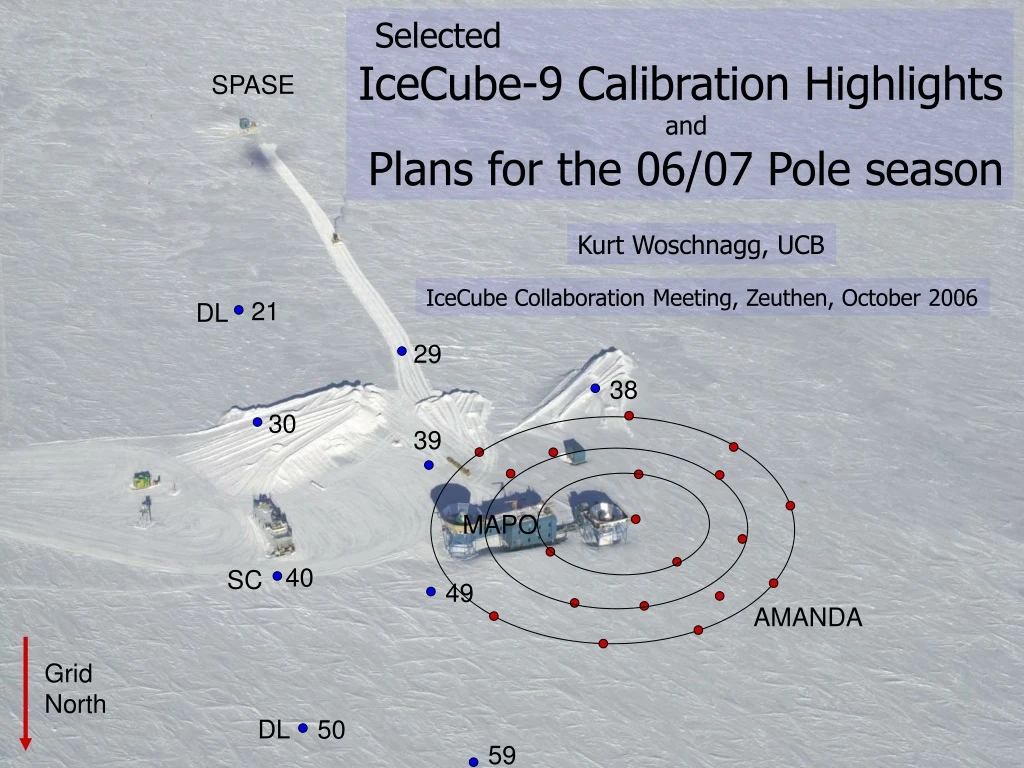
Selected IceCube-9 Calibration Highlights and Plans for the 06/07 Pole season SPASE Kurt Woschnagg, UCB IceCube Collaboration Meeting, Zeuthen, October 2006 21 DL 29 38 30 39 MAPO 40 SC 49 AMANDA Grid North DL 50 59
Selected Calibration Topics • Expectation Calibration • Geometry • Waveform Droop Correction • Ice Properties: • new ice model • deep bulk ice • dust layer tilt • reusable Dust Logger • hole ice: • 48/4 laser measurements • Bubble Camera • Standard Candle
IceCube Calibrations: advice from a prize winning physicist
IceCube Geometry Status • 9-string + IceTop geometry release on Jan 30 • Deployment data • Surface surveys • Verified with flashers and muons • Interstring geometry calibration (Chihwa Song) • AMANDA geometry shifted up 8.6 m after compressibility correction • Get your coordinates from offline database (I3Db)
survey data • drill tower • IceTop tanks/DOMs deployment data • pressure data • compressibility correction • well depth • DOM spacing drill data Hole profile Geometry Calibration(Stage 1) tower base plate Absolute (x,y,z) on surface well depth water surface String depth DOM spacing pressure sensors string depth in water Corrections (x,y) along string Absolute (x,y,z) for all DOMs DB bottom DOM (defines string depth)
38 39 D L Stage-2 geometry: interstring fits [Chihwa Song]
Stage-2 geometry: interstring fits Depth Offset (rel. to Stage-1 geometry) [m] String 39: offset = 0 [Chihwa Song]
Correcting waveforms for transformer droop [talk by Chris Wendt]
Correcting waveforms for transformer droop [Chris Wendt, Juande Zornoza]
Ice Model Evolution • Combine all known AMANDA measurements → “millennium” model (described in “the ice paper”) • 10-m bins • 800 to 2700 m (extrapolations using ice cores) • Impose higher depth resolution from dust logger data → “lordi” (preliminary release on 6/6/06) • 666 non-uniform depth bins • 1300 to 2450 m • Scattering/absorption table sent to Johan Lundberg for photonics table production (to be used in simulations) • Possible future ice models: • Add ash layers (cm-thin, highly absorbing, seen in dust logs) • Add dust layer tilt… Remember: non-layered ice models are not cool…
Start with raw DL data Hole 50 dust logger Start with bin=10 m if (in a bin) (max-min)/mean>0.1 then (for that bin) bin=bin/2 → 666 bins Scale linearly to scattering at 400 nm A new, high-res ice model: lordi
Extending the ice map for IceCube Need to complement AMANDA data
LOWINT flasher data analyzed so far Run# flasher <npe>@114m 31044 39:15 0.21 (30:15) 31046 39:39 0.52 (30:39) 31049 39:45 0.07 (30:45) 31055 39:55 0.09 (30:55) 31059 39:56 0.18 (30:56) 31061 39:57 0.06 (30:57) 31062 39:57 0.42 (30:57) 31064 39:58 0.15 (30:58) For all these runs: only the 6 horizontal LEDs flashing
Very preliminary results What’s next: 1. More data! 2. Systematics
The Dust Logger [Ryan Bay]
ice flow 3-D South Pole stratigraphy in IceCube 400 m colder dustier [Ryan Bay]
Dust logs correlate with Ice Properties A B dust layers C D clearest ice
Hole 21 vs. Hole 50 logs and dust layer “tilt” First measure of dust layer tilt over ~400 m Small enough not to trigger immediate modification of ice modeling: keep layers horizontal, for now…
Reusable Dust Logger • Reconfigured DL hole logger on RG winch • Log just before deployment • Advantages: • Higher data quality • Duplicate log of hole • Save $ • Standby use • Plan for 06/07 season: • Log 1 or 2 holes [talk by Ryan Bay]
Air bubbles trapped in the refrozen ice column increase scattering close to the modules → Make angular acceptance more isotropic →Uncertainty is major systematic in many analyses hole ice (trapped bubbles) bulk ice (some dust) All 20 OMs on AMANDA string 4 have a diffusing fiber ball connected to surface laser String 4 will be ~15 m from IceCube string 48 (9th string in 06/07)
Reducing Systematics through Calibrations Measure in situ? Reduced with photonics! AMANDA papers
[Michelangelo D’Agostino] 1 2 3 4 5 6 cable 1 2 3 4 5 6 cable An illustration of the complexity of the hole ice situation… Average waveforms at DOM above flashing DOM Vertical LED’s Horizontal LED’s black = water; green/blue = ice Bubble formation appears to be non-azimuthally symmetric…
This Season: the 48/4 hole ice studies String 48 will be deployed near center of AMANDA Within ~10-15 m of AMANDA string 4 String 4 has optical fibers with diffuser balls at every OM location Use surface YAG laser and take interstring data in water, while freezing, and in ice Plan exists, was discussed in Ver/Cal session 20 m 17 m ~15 m -4 48
Hole ice studies with a “bubble camera” Bubble Camera: Two camera modules in regular DOM spheres (one hemisphere is polished) One camera looking up, one looking down Looking at DOM60 (2-3 m above), eye charts Possible quantitative measurements: - Attenuation length - Bubble distribution - Time constants for transition from air bubbles (scattering) to clathrate crystals (invisible) [talk by Michelangelo D’Agostino]
un-polished sphere polished sphere no sphere
overlapping energy region useful for cross-calibration depends on brightness setting,# of LEDs, pulse width flashers SC I SC II Cascade Calibration: in situ light sources cascade energy* GeV TeV PeV EeV *applying rule-of-thumb: 105 photons/GeV • Complications to keep in mind: • ice properties ~20% worse at 337 nm than at 405 nm • glass transmission at 337 nm only ~1/3 of that at 405 nm • hole ice modifies emission pattern • real cascades have Cherenkov spectrum • real cascades are not point sources
Standard Candle II (next season) String 57, between DOMs 12 & 13 Pointing down 1812.5 m Standard Candle I String 40 Between DOMs 22 and 23 Pointing up
SC preliminary analysis: angular profile ~40° cone observed on neighboring strings [Michelangelo D’Agostino]
57 Standard Candles in IceCube
Summary of Season 06/07 Calibrations dust logging standard candle bubble camera hole ice 48/4