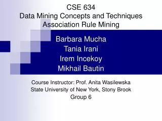
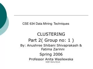
CSE 634 Data Mining Techniques
CSE 634 Data Mining Techniques. Presentation on Neural Network Jalal Mahmud ( 105241140) Hyung-Yeon, Gu (104985928) Course Teacher : Prof. Anita Wasilewska State University of New York at Stony Brook. References. Data Mining Concept and Techniques (Chapter 7.5)


CSE 634 Data Mining Techniques
E N D
Presentation Transcript
CSE 634 Data Mining Techniques Presentation on Neural Network Jalal Mahmud ( 105241140) Hyung-Yeon, Gu(104985928) Course Teacher : Prof. Anita Wasilewska State University of New York at Stony Brook
References • Data Mining Concept and Techniques (Chapter 7.5) [Jiawei Han, Micheline Kamber/Morgan Kaufman Publishers2002] • Professor Anita Wasilewska’s lecture note • www.cs.vu.nl/~elena/slides03/nn_1light.ppt • Xin Yao Evolving Artificial Neural Networkshttp://www.cs.bham.ac.uk/~xin/papers/published_iproc_sep99.pdf • informatics.indiana.edu/larryy/talks/S4.MattI.EANN.ppt • www.cs.appstate.edu/~can/classes/ 5100/Presentations/DataMining1.ppt • www.comp.nus.edu.sg/~cs6211/slides/blondie24.ppt • www.public.asu.edu/~svadrevu/UMD/ThesisTalk.ppt • www.ctrl.cinvestav.mx/~yuw/file/afnn1_nnintro.PPT
Overview • Basics of Neural Network • Advanced Features of Neural Network • Applications I-II • Summary
Basics of Neural Network • What is a Neural Network • Neural Network Classifier • Data Normalization • Neuron and bias of a neuron • Single Layer Feed Forward • Limitation • Multi Layer Feed Forward • Back propagation
Biologically motivated approach to machine learning Neural Networks What is a Neural Network? Similarity with biological network Fundamental processing elements of a neural network is a neuron 1.Receives inputs from other source 2.Combines them in someway 3.Performs a generally nonlinear operation on the result 4.Outputs the final result
Similarity with Biological Network • Fundamental processing element of a neural network is a neuron • A human brain has 100 billion neurons • An ant brain has 250,000 neurons
Neural Network • Neural Network is a set of connected INPUT/OUTPUT UNITS, where each connection has a WEIGHT associated with it. • Neural Network learning is also called CONNECTIONIST learning due to the connections between units. • It is a case of SUPERVISED, INDUCTIVE or CLASSIFICATION learning.
Neural Network • Neural Network learns by adjusting the weights so as to be able to correctly classify the training data and hence, after testing phase, to classify unknown data. • Neural Network needs long time for training. • Neural Networkhas a high tolerance to noisy and incomplete data
Neural Network Classifier • Input: Classification data It contains classification attribute • Data is divided, as in any classification problem. [Training data and Testing data] • All data must be normalized. (i.e. all values of attributes in the database are changed to contain values in the internal [0,1] or[-1,1]) Neural Network can work with data in the range of (0,1) or (-1,1) • Two basic normalization techniques [1] Max-Min normalization [2] Decimal Scaling normalization
Data Normalization [1] Max- Min normalization formula is as follows: [minA, maxA , the minimun and maximum values of the attribute A max-min normalization maps a value v of A to v’ in the range {new_minA, new_maxA} ]
Example of Max-Min Normalization Max- Min normalization formula Example:We want to normalize data to range of the interval [0,1]. We put: new_max A= 1, new_minA =0. Say, max A was 100 and min A was 20 ( That means maximum and minimum values for the attribute ). Now, if v = 40 ( If for this particular pattern , attribute value is 40 ), v’ will be calculated as , v’ = (40-20) x (1-0) / (100-20) + 0 => v’ = 20 x 1/80 => v’ = 0.4
Decimal Scaling Normalization [2]Decimal Scaling Normalization Normalization by decimal scaling normalizes by moving the decimal point of values of attribute A. Here j is the smallest integer such that max|v’|<1. Example : A – values range from -986 to 917. Max |v| = 986. v = -986 normalize to v’ = -986/1000 = -0.986
One Neuron as a Network • Here x1 and x2 are normalized attribute value of data. • y is the output of the neuron , i.e the class label. • x1 and x2 values multiplied by weight values w1 and w2 are input to the neuron x. • Value of x1 is multiplied by a weight w1 and values of x2 is multiplied by a weight w2. • Given that • w1 = 0.5 and w2 = 0.5 • Say value of x1 is 0.3 and value of x2 is 0.8, • So, weighted sum is : • sum= w1 x x1 + w2 x x2 = 0.5 x 0.3 + 0.5 x 0.8 = 0.55
One Neuron as a Network • The neuron receives the weighted sum as input and calculates the output as a function of input as follows : • y = f(x) , where f(x) is defined as • f(x) = 0 { when x< 0.5 } • f(x) = 1 { when x >= 0.5 } • For our example, x ( weighted sum ) is 0.55, so y = 1 , • That means corresponding input attribute values are classified in class 1. • If for another input values , x = 0.45 , then f(x) = 0, • so we could conclude that input values are classified to class 0.
Bias of a Neuron • We need the bias value to be added to the weighted sum ∑wixi so that we can transform it from the origin. v = ∑wixi + b, here b is the bias x1-x2= -1 x2 x1-x2=0 x1-x2= 1 x1
w0 x0 = +1 x1 W1 Activation function v Output class y Input Attribute values x2 w2 Summing function weights xm wm Bias as extra input
Neuron with Activation • The neuron is the basic information processing unit of a NN. It consists of: 1 A set of links, describing the neuron inputs, with weightsW1, W2, …, Wm 2. An adder function (linear combiner) for computing the weighted sum of the inputs (real numbers): 3 Activation function : for limiting the amplitude of the neuron output.
Why We Need Multi Layer ? • Linear Separable: • Linear inseparable: • Solution?
A Multilayer Feed-Forward Neural Network Output Class Output nodes Hidden nodes wij - weights Input nodes Network is fully connected Input Record : xi
Neural Network Learning • The inputs are fed simultaneously into the input layer. • The weighted outputs of these units are fed into hidden layer. • The weighted outputs of the last hidden layer are inputs to units making up the output layer.
A Multilayer Feed Forward Network • The units in the hidden layers and output layer are sometimes referred to as neurodes, due to their symbolic biological basis, or as output units. • A network containing two hidden layers is called a three-layer neural network, and so on. • The network is feed-forward in that none of the weights cycles back to an input unit or to an output unit of a previous layer.
A Multilayered Feed – Forward Network • INPUT: records without class attribute with normalized attributes values. • INPUT VECTOR: X = { x1, x2, …. xn} where n is the number of (non class) attributes. • INPUT LAYER – there are as many nodes as non-class attributes i.e. as the length of the input vector. • HIDDEN LAYER – the number of nodes in the hidden layer and the number of hidden layers depends on implementation.
A Multilayered Feed–Forward Network • OUTPUT LAYER – corresponds to the class attribute. • There are as many nodes as classes (values of the class attribute). k= 1, 2,.. #classes • Network is fully connected, i.e. each unit provides input • to each unit in the next forward layer.
Classification by Back propagation • Back Propagation learns by iteratively processing a set of training data (samples). • For each sample, weights are modified to minimize the error between network’s classification and actual classification.
Steps in Back propagation Algorithm • STEP ONE: initialize the weights and biases. • The weights in the network are initialized to random numbers from the interval [-1,1]. • Each unit has a BIAS associated with it • The biases are similarly initialized to random numbers from the interval [-1,1]. • STEP TWO: feed the training sample.
Steps in Back propagation Algorithm ( cont..) • STEP THREE: Propagate the inputs forward; we compute the net input and output of each unit in the hidden and output layers. • STEP FOUR: back propagate the error. • STEP FIVE: update weights and biases to reflect the propagated errors. • STEP SIX: terminating conditions.
- x0 w0j x1 w1j f å output y xn wnj Input vector x weight vector w weighted sum Activation function Propagation through Hidden Layer ( One Node ) Bias j • The inputs to unit j are outputs from the previous layer. These are multiplied by their corresponding weights in order to form a weighted sum, which is added to the bias associated with unit j. • A nonlinear activation function f is applied to the net input.
Propagate the inputs forward • For unit j in the input layer, its output is equal to its input, that is, • for input unit j. • The net input to each unit in the hidden and output layers is computed as follows. • Given a unit j in a hidden or output layer, the net input is where wij is the weight of the connection from unit i in the previous layer to unit j; Oi is the output of unit I from the previous layer; is the bias of the unit
Propagate the inputs forward • Each unit in the hidden and output layers takes its net input and then applies an activation function. The function symbolizes the activation of the neuron represented by the unit. It is also called a logistic, sigmoid, or squashing function. • Given a net input Ij to unit j, then Oj = f(Ij), the output of unit j, is computed as
Back propagate the error • When reaching the Output layer, the error is computed and propagated backwards. • For a unit k in the output layer the error is computed by a formula: Where O k – actual output of unit k ( computed by activation function. Tk – True output based of known class label; classification of training sample Ok(1-Ok) – is a Derivative ( rate of change ) of activation function.
Back propagate the error • The error is propagated backwards by updating weights and biases to reflect the error of the network classification . • For a unit j in the hidden layer the error is computed by a formula: where wjk is the weight of the connection from unit j to unit k in the next higher layer, and Errk is the error of unit k.
Update weights and biases • Weights are updated by the following equations, where l is a constant between 0.0 and 1.0 reflecting the learning rate, this learning rate is fixed for implementation. • Biases are updated by the following equations
Update weights and biases • We are updating weights and biases after the presentation of each sample. • This is called case updating. • Epoch --- One iteration through the training set is called an epoch. • Epoch updating ------------ • Alternatively, the weight and bias increments could be accumulated in variables and the weights and biases updated after all of the samples of the training set have been presented. • Case updating is more accurate
Terminating Conditions • Training stops • All in the previous epoch are below some threshold, or • The percentage of samples misclassified in the previous epoch is below some threshold, or • a pre specified number of epochs has expired. • In practice, several hundreds of thousands of epochs may be required before the weights will converge.
Backpropagation Formulas Output vector Output nodes Hidden nodes wij Input nodes Input vector: xi
Example of Back propagation Input = 3, Hidden Neuron = 2 Output =1 Initialize weights : Random Numbers from -1.0 to 1.0 Initial Input and weight
Example ( cont.. ) • Bias added to Hidden • + Output nodes • Initialize Bias • Random Values from • -1.0 to 1.0 • Bias ( Random )
Net Input and Output Calculation = 0.332 = 0.525 = 0.475
Calculation of weights and Bias Updating Learning Rate l =0.9
Advanced Features of Neural Network • Training with Subsets • Modular Neural Network • Evolution of Neural Network
Variants of Neural Networks Learning • Supervised learning/Classification • Control • Function approximation • Associative memory • Unsupervised learning or Clustering
Training with Subsets • Select subsets of data • Build new classifier on subset • Aggregate with previous classifiers • Compare error after adding classifier • Repeat as long as error decreases
Subset 1 NN 1 Subset 2 NN 2 The Whole Dataset Split the dataset into subsets that can fit into memory Subset 3 NN 3 Subset n NN n A Single Neural Network Model Training with subsets . . .
Modular Neural Network • Modular Neural Network • Made up of a combination of several neural networks. The idea is to reduce the load for each neural network as opposed to trying to solve the problem on a single neural network.
Evolving Network Architectures • Small networks without a hidden layer can’t solve problems such as XOR, that are not linearly separable. • Large networks can easily overfit a problem to match the training data, limiting their ability to generalize a problem set.
Constructive vs Destructive Algorithm • Constructive algorithms take a minimal network and build up new layers nodes and connections during training. • Destructive algorithms take a maximal network and prunes unnecessary layers nodes and connections during training.
Training Process of the MLP • The training will be continued until the RMS is minimized. ERROR Local Minimum Local Minimum Global Minimum W (N dimensional)
Faster Convergence • Back prop requires many epochs to converge • Some ideas to overcome this • Stochastic learning • Update weights after each training example • Momentum • Add fraction of previous update to current update • Faster convergence