Directed Acyclic Graphs

1. Directed Acyclic Graphs David A. Bessler Texas A&M University November 20, 2002 Universidad Internacional del Ecuador Quito, Ecuador

2. Outline Introduction Causal Forks Inverted Causal Forks D-separation Markov Property The Adjustment Problem  Policy Modeling PC Algorithm 

3. Outline Continued Example: Traffic Fatalities Correlation and Partial Correlation Forecasting Traffic Fatalities More Examples: US Money, Prices and Income  World Stock Markets Conclusion 

4. Motivation Oftentimes we are uncertain about which variables are causal in a modeling effort. Theory may tell us what our fundamental causal variables are in a controlled system; however, it is common that our data may not be collected in a controlled environment. In fact we are rarely involved with the collection of our data.

5. Observational Data In the case where no experimental control is present in the generation of our data, such data are said to be observational (non-experimental) and usually secondary, not collected explicitly for our purpose but rather for some other primary purpose.

6. Use of Theory Theory is a good potential source of information about direction of causal flow. However, theory usually invokes the ceteris paribus condition to achieve results. Data are usually observational (non-experimental) and thus the ceteris paribus condition may not hold. We may not ever know if it holds because of unknown variables operating on our system (see Malinvaud’s econometric text).

7. Experimental Methods If we do not know the "true" system, but have an approximate idea that one or more variables operate on that system, then experimental methods can yield appropriate results. Experimental methods work because they use randomization, random assignment of subjects to alternative treatments, to account for any additional variation associated with the unknown variables on the system.

8. Directed Graphs Can Be Used To Represent Causation Directed graphs help us assign causal flows to a set of observational data. The problem under study and theory suggests certain variables ought to be related, even if we do not know exactly how; i.e. we don’t know the "true" system.

9. Causal Models Are Well Represented By Directed Graphs One reason for studying causal models, represented here as X  Y, is to predict the consequences of changing the effect variable (Y) by changing the cause variable (X). The possibility of manipulating Y by way of manipulating X is at the heart of causation. Hausman (1998, page 7) writes: “Causation seems connected to intervention and manipulation: One can use causes to ‘wiggle’ their effects.”

10. We Need More Than Algebra To Represent Cause Linear algebra is symmetric with respect to the equal sign. We can re-write y = a + bx as x = -a/b +(1/b)y. Either form is legitimate for representing the information conveyed by the equation. A preferred representation of causation would be the sentence x  y, or the words: “if you change x by one unit you will change y by b units, ceteris paribus.” The algebraic statement suggests a symmetry that does not hold for causal statements.

11. Arrows Carry the Information An arrow placed with its base at X and head at Y indicates X causes Y: X  Y. By the words “X causes Y” we mean that one can change the values of Y by changing the values of X. Arrows indicate a productive or genetic relationship between X and Y. Causal Statements are asymmetric: x  y is not consistent with y  x.

12. Problems with Predictive Definitions of Cause Definition of the word “cause” that focus on prediction alone, without distinguishing between intervention (first) and subsequent realization, may mistakenly label as causal variables that are associated only through an omitted variable. Prediction is one attribute of the word “cause.” We must be careful not to make it the only attribute (more or less a summary of Bunge 1959).

13. Granger-type Causality For example, Granger-type causality (Granger 1980) focuses solely on prediction, without considering intervention. If we can predict Y better by using past values of X than by not using past values of X , then X Granger-causes Y. The consequences of such focus is to open oneself up to the frustration of unrealized expectations by attempting policy on the wrong set of variables.

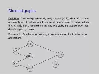
14. Graph A graph is an ordered triple <V,M,E>. V is a non-empty set of vertices (variables). M is a non-empty set of marks (symbols attached to the end of undirected edges). E is a set of ordered pairs. Each member of E is called an edge.

15. Vertices are variables; Edges are lines Vertices connected by an edge are said to be adjacent. If we have a set of vertices {A,B,C,D} the undirected graph contains only undirected edges (e.g., A  B). A directed graph contains only directed edges: C  D.

16. Directed Acyclic Graphs (DAGs) A directed acyclic graph is a directed graph that contains no directed cyclic paths. An acyclic graph has no path that leads away from a variable only to return to that same variable. The path A  B  C  A is labeled “cyclic” as here we move from A to B, but then return to A by way of C.

17. Graphs and Probabilities of Variables Directed acyclic graphs are pictures (illustrations) for representing conditional independence as given by the recursive decomposition: n Pr(v1,v2 …vn-1,vn ) =  Pr( vi | pai ) i=1 where Pr is the probability of vertices (variables) v1, v2, v3, ... vn and pai the realization of some subset of the variables that precede (come before in a causal sense) vi in order (v1, v2, v3, ... vn), and the symbol  represents the product operation, with index of operation denoted below (start) and above (finish) the symbol. Think of pai as the parent of variable i.

18. D-Separation Let X, Y and Z be three disjoint subsets of variables in a directed acylic graph G, and let p be any path between a vertex [variable] in X and a vertex [variable] in Y, where by 'path' we mean any succession of edges, regardless of their directions. Z is said to block p if there is a vertex w on p satisfying one of the following: • (i) w has converging arrows along p, and neither w nor any of its descendants are on Z or • (ii) w does not have converging arrows along p, and w is in Z. Furthermore, Z is said to d-separate X from Y on graph G, written (X  Y | Z)G , if and only if Z blocks every path from a vertex [variable] in X to a vertex [variable] in Y.

19. Graphs and D-Separation Geiger, Verma and Pearl (1990) show that there is a one-to-one correspondence between the set of conditional independencies, X  Y | Z, implied by the above factorization and the set of triples, X, Y, Z, that satisfy the d-separation criterion in graph G. If G is a directed acyclic graph with vertex set V, if A and B are in V and if H is also in V, then G linearly implies the correlation between A and B conditional on H is zero if and only if A and B are d-separated given H.

20. Colliders (Inverted Fork) Consider three variables (vertices): A, B and C. A variable is a collider if arrows converge on it: A  B  C. The vertex B is a collider, A and C are d-separated, given the null set. Intuitively, think of two trains one starting at A, the other at C. Both move toward B. Unconditionally, they will crash at B. However, if we condition on B, (if we build a switch station at B with side tracks), we open-up the flow from A to C. Conditioning on B makes A and C d-connected (directionally connected).

21. Conditioning on Children (of colliders) Opens Up Information Flows Too! Amend the above graph given above to include variable D, as a child of B, such that: A  B  C  D If we condition on D rather than B, we, as well, open up the flow between A and C (Pearl, 2000 p.17). This illustrates the (i) component of the definition given above.

22. Common Causes (causal fork) Say we have three vertices K, L and M, described by the following graph: K  L  M. Here L is a common cause of K and M. The unconditional association (correlation) between K and M will be non-zero, as they have a common cause L. However, if we condition on L (know the value of L), the association between K and M disappears (Pearl, 2000, p.17). Conditioning on common causes blocks the flow of information between effects.

23. Causal chains Finally, if our causal path is one of a chain (causal chain), condition (ii) in the above definition again applies. If D causes E and E causes F, we have the representational flow: D E F. The unconditional association (correlation) between D and F will be non-zero, but the association (correlation) between D and F conditional on E will be zero. (For those in the audience familiar with Box and Jenkins’ time series methods, this is a property they exploited in testing for AR models)

24. Example of an Inverted Causal Fork In the example we study below we take data from Peltzman (Jo. Political Economy 1976). This is a study of Traffic Fatalities in the U.S. over the period 1947 – 1972. Roh, Bessler and Gilbert (1997) find the following (not a surprise):  Speed(t)  Alcohol Consumption(t)  Traffic Fatalities(t)

25. What Should We Expect Based On The Previous Directed Graph? Here year to year changes in speed and year to year changes in alcohol consumption are direct causes of year to year changes in traffic fatalities. The graph is an inverted fork. So,…, we should expect to see that  Speed and  Alcohol Consumption are not related in unconditional tests of association. However, if we condition on  Traffic Fatalities , we should see a non-zero measure of association between  Speed and  Alcohol Consumption.

26. OLS Regressions On An Inverted Fork(use ols to measure association) Regression #1:  Speed(t) = .01 - .01*( Alcohol Consumption(t)) (.002) (.053) Estimated standard errors of the coefficients are in ( ). Based on this regression we would say  Speed(t) and  Alcohol Consumption(t) are not related (note: -.01/.053 < 2.0).

27. OLS Regressions On An Inverted Fork:Now We Condition on the Effect (traffic fatalities) Regression #2:  Speed(t) = .01 - .11*( Alcohol Consumption(t)) (.002) (.051) + .15 * ( Traffic Fatalities(t)) (.046) Here conditioning on the common effect makes the two causes dependent (note: -.11/.051 > 2.0).

28. Example of a Causal Chain In another example, consider the relationship among GDP, Poverty and Malnutrition. Based on World Bank data for 80 less developed countries, we find: GDP  Poverty  Malnutrition We expect, from the directed graph theory given above, Malnutrition and GDP will be related in unconditional tests. However, if we condition on poverty they should be unrelated. Let’s see!

29. Regressions with Causal Chains Regression #1 (for i=1, …, 80 countries) Malnutrition(i) = 24.18 - .003* GDP(i) (1.91) (.0006) Note the t-ratio of -.003/.0006 = -5.38 suggests that GDP is an important variable in moving levels of malnutrition.

30. Regressions with Causal Chains, continued. Regression #2 (for i=1, …, 80 countries) Malnutrition(i) = 7.52 - .0013* GDP(i) (2.09) (.0007) + .289 * Poverty(i) (.055) Note the t-ratio of -.0013/.0007 = -1.78 suggests (if we are 5% er’s) that GDP is not informative with respect to malnutrition if we have information about a country’s poverty levels.

31. Markov Property Key to understanding these ideas is that d-separation allows us to write the probability of our variables X,Y, and Z in terms of the product of the conditional probabilities on each variable (X,Y, or Z), where the conditioning factor is the immediate parent of each variable. We do not have to condition on grandparents, great grandparents, aunts, uncles or children. (It is helpful and valid to refer to genealogical analogies when thinking about conditioning information.)

32. Some probabilities The following directed graphs have these associated probability factorizations: A  B  C ; Pr(A,B,C) = Pr(A) Pr(C)Pr(B|C,A) D  E  F ; Pr(D,E,F) = Pr(D)Pr(E|D)Pr(F|E) GHI J; Pr(G,H,I,J) = Pr(G)Pr(J)Pr(H|G)Pr(I|J,H) P Q ; Pr(P,Q) = Pr(P)Pr(Q) Here Pr(.) refers to the probability of the variable(s) in parentheses

33. Adjustment Problem(from Pearl 2000) What must I measure if I want to know how X affects Y? Z1 Z2 Z3 Z4 Z5 Z6 Z7 Z8 Z9 Z10 X Z11 Y Original Causal Graph Illustrating the “Adjustment Problem”

34. D-Separation is Key to Solving the Adjustment Problem Ask the question: can I get back to Y via the ancestors of X without running into converging arrows? Yes! I can take several paths from X to Y through X’s ancestors: X – Z3 – Z1– Z4 – Z7 – Y X – Z6 – Z4– Z7 – Y X – Z6 – Z4– Z2 – Z5– Z9 – Y X – Z6 – Z4– Z2 – Z7 – Y I have to condition on variables to “block” the path back to Y from X. There are several possibilities: It looks like Z7 and Z9 are two. Below we give six steps for solving the “adjustment problem”.

35. Step 1. Z7 and Z9 should be non-descendants of X Z1 Z2 Z3 Z4 Z5 Z6 Z7 Z8Z9 Z10 X Z11 Y Z11 will not work as it is a child of X.

36. Step 2. Delete all non-ancestors of {X,Y and Z}. Z1 Z2 Z3 Z4 Z5 Z6 Z7 Z8 Z9 Z10 X Z11 Y Here Z is the set of candidate “blocking” variables Z = {Z7and Z9}.

37. Step 3. Delete all arcs emanating from X. Z1 Z2 Z3 Z4 Z5 Z6 Z7 Z8 Z9 Z10 X Z11 Y Here we will remove the X  Z11 edge, as Z11 is a child of X.

38. Step 4. Connect any two parents sharing a common child. Z1 Z2 Z3 Z4 Z5 Z6 Z7 Z8Z9 Z10 X Z11 Y Here we will use dotted lines to connect parents with a common child

39. Step 5. Strip arrow-heads from all edges Z1 Z2 Z3 Z4 Z5 Z6 Z7 Z8Z9 Z10 X Z11 Y

40. Step 6. Delete Lines into and out of Z7 and Z9 Z1 Z2 Z3 Z4 Z5   We cannot get Z6 Z7from X to Y Z8Z9 Z10 X Z11 Y Here we delete all lines into the variables that we wish to condition on, Z7 and Z9.

41. Test Test: if X is disconnected from Y in the remaining graph, then Z7 and Z9 are sufficient measurements to condition on. By “disconnected” we mean that we cannot get from X to Y via the remaining lines. Z7 and Z9 pass the test. So we can perform ols regression of Y on X, Z7 and Z9 to find an unbiased estimate of the effect of X on Y.

42. Another candidate: Let’s Try Z4 all by Itself. If we try just Z4 as a sole candidate variable to condition on, our last figure will be amended as follows: Z1 Z2 Z3 Z4 Z5 Z6 Z7 Z8 Z9 Clearly Z4 Z10 will not work X Z11 Y

43. Why does Z4 fail our test in the previous slide? Because Z4 opens up the path between Z1 and Z2. Remember our speed, alcohol and traffic fatalities example, slides 24 – 27. If we run an ols regression of Y on X and Z4 we would find biased estimates of the coefficient associated with X. X will be correlated with errors in Y. We say there is a “backdoor path” between X and Y that will give us biased parameter estimates of the effect of X on Y.

44. Policy and Directed Graphs Consider the following simple graph:   X  Y  U  We observe X in an uncontrolled setting and we are interested in manipulating Y by setting the value of X. The inference task we have as economists is to move from a sample obtained from a distribution associated with passive observation to conclusions about the distribution that would obtain if a particular policy is imposed. Policy is thus asking questions about counterfactuals. What values will Y take on if we force X to take on a value of Xf=1 ? (here we use the notation that X is forced to have a value of 1 as Xf=1).

45. Simple Example of Policy with Exogenous Variable X • Consider the table which is based on the graph given above, where Y = X + U Passive Observations | Forced or Policy Induced X U Y Xf UXf=1 YXf=1 1 0 1 1 0 1 1 1 2 1 1 2 1 2 3 1 2 3 2 0 2 1 0 1 2 1 3 1 1 2 2 2 4 1 2 3 Notice how Y behaves when we force a value on X (X=1).

46. What were we suppose to see in the previous table? In the above table, Y, under passive observation when X=1, has the same distribution as YXf=1. Look back at the table. Here X is a parent of Y and there is no backdoor path from X to Y (say via U). A policy analyst may conclude that knowing how X and Y are related in this uncontrolled (passive) setting is sufficient for predicting how they will behave in policy settings.

47. A case where we must be careful   V X Y U Here we have a variable V that causes both X and U. Will knowledge of how X and Y behave in passive settings be sufficient for predicting how they will behave in a policy setting?

48. Consider the following: Let: Y = X + U ; X = V and U = V Passive Observations | Forced or Policy Induced V X U Y V Xf=1 UXf=1 YXf=1 1 1 1 2 1 1 1 2 1 1 1 2 1 1 1 2 1 1 1 2 1 1 1 2 2 2 2 4 2 1 2 3 2 2 2 4 2 1 2 3 2 2 2 4 2 1 2 3 Notice here that when X=1 in the unforced setting our distribution on Y is 2,2,2,4,4,4. However, when we force X=1 our distribution on Y is sometimes 2, and sometimes 3, but never 4. Under the policy setting on X we cannot ignore V. We have to have it in our model, else we will have policy results which are not well predicted through knowledge of X and Y (passively observed).

49. Results on Traffic Fatalities We find the following relationship among traffic fatalities, alcohol consumption and income. alcohol consumption(t) income(t) traffic fatalities(t) This graph along with our work above on policy analysis suggests that it is not enough to understand the alcohol – traffic fatalities link, but we must as well understand how income levels contribute to the problem.

50. Consider the Following Two Regressions Regression # 1: (Ignore the Income connection) TF(t) = .015 + .608 AC(t) : R2 = .38 (.009) (.200) Regression # 2: (Include Income with Alcohol Consumption) TF(t) = -.005 + .338 AC(t) + 1.055 IN(t) ; R2 = .68 (.008) (.160) (.276)