Scheduling in Batch Systems
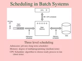
Scheduling in Batch Systems. Three level scheduling Admission: job mix (long term scheduler) Memory: degree of multiprogramming (medium term) CPU Scheduler: algorithm to choose ready process to run (short term). Basic Concepts. Maximum CPU utilization obtained with multiprogramming

Scheduling in Batch Systems
E N D
Presentation Transcript
Scheduling in Batch Systems Three level scheduling Admission: job mix (long term scheduler) Memory: degree of multiprogramming (medium term) CPU Scheduler: algorithm to choose ready process to run (short term)
Basic Concepts • Maximum CPU utilization obtained with multiprogramming • CPU–I/O Burst Cycle – Process execution consists of a cycle of CPU execution and I/O wait. • CPU burst distribution
Histogram of CPU-burst Times • Lots of short CPU activities • Few CPU intensive
CPU Scheduler • Selects from among the processes in memory that are ready to execute, and allocates the CPU to one of them. • CPU scheduling decisions may take place when a process: 1. Switches from running to waiting state. 2. Switches from running to ready state. 3. Switches from waiting to ready. 4. Terminates. • Scheduling under 1 and 4 is nonpreemptive. • All other scheduling is preemptive.
Dispatcher • Dispatcher module gives control of the CPU to the process selected by the short-term scheduler; this involves: • switching context • switching to user mode • jumping to the proper location in the user program to restart that program • Dispatch latency – time it takes for the dispatcher to stop one process and start another running.
Scheduling Criteria • CPU utilization – percentage of time the CPU is executing a process (* more on next slide *) • Throughput – # of processes that complete their execution per time unit • Turnaround time – amount of time to execute a particular process • Waiting time – amount of time a process has been waiting in the ready queue • Response time – amount of time it takes from when a request was submitted until the first response is produced, not output (for time-sharing environment)
CPU Utilization • Keep the CPU as busy as possible • Load on system affects level of utilization • High level of utilization is easier to reach on heavily loaded system • On single-user system, CPU utilization is not very important • On time-shared system, CPU utilization may be primary consideration
Optimization Criteria • Max CPU utilization • Max throughput • Min turnaround time • Min waiting time • Min response time
Scheduling Algorithms • Non-preemptive • Process retains control of CPU until process blocks or is terminated • Good for batch jobs when response time is of little concern • Common: FCFS, SJF • Preemptive • Scheduler may preempt a process before it blocks or terminates, in order to allocate CPU to another process • Necessary on interactive systems • Common: SRT, RR
P1 P2 P3 0 24 27 30 First-Come, First-Served (FCFS) Scheduling ProcessBurst Time P1 24 P2 3 P3 3 • Suppose that the processes arrive in the order: P1 , P2 , P3 The Gantt Chart for the schedule is: • Waiting time for P1 = 0; P2 = 24; P3 = 27 • Average waiting time: (0 + 24 + 27)/3 = 17
P2 P3 P1 0 3 6 30 FCFS Scheduling (Cont.) Suppose that the processes arrive in the order P2 , P3 , P1 . • The Gantt chart for the schedule is: • Waiting time for P1 = 6;P2 = 0; P3 = 3 • Average waiting time: (6 + 0 + 3)/3 = 3 • Much better than previous case. • Convoy effect short process behind long process • Short jobs suffer • Favors CPU bound processes
Shortest-Job-First (SJF) Scheduling • Associate with each process the length of its next CPU burst. Use these lengths to schedule the process with the shortest time. Tie breaker via FCFS. • Two schemes: • nonpreemptive – once CPU given to the process it cannot be preempted until completes its CPU burst. • preemptive – if a new process arrives with CPU burst length less than remaining time of current executing process, preempt. This scheme is know as the SJF-preemptive or Shortest-Remaining-Time-First (SRT or SRTF). • SJF is optimal – gives minimum average waiting time for a given set of processes.
P1 P3 P2 P4 0 3 7 8 12 16 Example of Non-Preemptive SJF Process Arrival TimeBurst Time P1 0.0 7 P2 2.0 4 P3 4.0 1 P4 5.0 4 • SJF (non-preemptive) • Average waiting time = (0 + 6 + 3 + 7)/4 = 4
P1 P2 P3 P2 P4 P1 11 16 0 2 4 5 7 Example of Preemptive SJF Process Arrival TimeBurst Time P1 0.0 7 P2 2.0 4 P3 4.0 1 P4 5.0 4 • SJF (preemptive) • Average waiting time = (9 + 1 + 0 +2)/4 = 3 • Consider the context switching overhead cost
SJF • Favors short jobs over long • Constant arrival of small jobs can lead to starvation of long jobs
Priority Scheduling • A priority number (integer) is associated with each process • Base on process characteristic (memory usage, I/O frequency) • Base on user • Base on usage cost (CPU time for higher priority costs more) • User or administrator assigned (static) • May be dynamic (e.g., changing with amount of time running)
Priority Scheduling (continued) • The CPU is allocated to the process with the highest priority (smallest integer highest priority). • Preemptive • nonpreemptive • SJF is a priority scheduling algorithm where priority is the predicted next CPU burst time. • Problem Starvation – low priority processes may never execute. • Solution Aging – as time progresses increase the priority of the process.
Round Robin (RR) • Each process gets a small unit of CPU time (time quantum), usually 10-100 milliseconds. After this time has elapsed, the process is preempted and added to the end of the ready queue. (Interval timer generates interrupt.) • If there are n processes in the ready queue and the time quantum is q, then each process gets 1/n of the CPU time in chunks of at most q time units at once. No process waits more than (n-1)q time units. • Performance • q large FIFO • q small good response time; however, q must be large with respect to context switch, otherwise overhead is too high.
P1 P2 P3 P4 P1 P3 P4 P1 P3 P3 0 20 37 57 77 97 117 121 134 154 162 Ex. of RR with Time Quantum = 20 ProcessBurst Time P1 53 P2 17 P3 68 P4 24 • The Gantt chart is: • Typically, higher average turnaround than SJF, but better response.
Treating All Jobs the Same • These algorithms basically treat all jobs the same • Each algorithm favors a certain kind of process • To address this deficiency, multilevel feedback queues customize the scheduling of processes based on the process’s performance characteristics by utilizing 2 or more scheduling algorithms • Flexible • Complex
Multilevel Queue • Ready queue is partitioned into separate queues:foreground (interactive)background (batch) • Each queue has its own scheduling algorithm, foreground – RRbackground – FCFS • Scheduling must be done between the queues. • Fixed priority scheduling; (i.e., serve all from foreground then from background). Possibility of starvation. • Time slice – each queue gets a certain amount of CPU time which it can schedule amongst its processes; i.e., 80% to foreground in RR • 20% to background in FCFS
Multilevel Feedback Queue • A process can move between the various queues; aging can be implemented this way. • Multilevel-feedback-queue scheduler defined by the following parameters: • number of queues • scheduling algorithms for each queue • method used to determine when to upgrade a process • method used to determine when to demote a process • method used to determine which queue a process will enter when that process needs service
Example of Multilevel Feedback Queue • Three queues: • Q0 – time quantum 8 milliseconds • Q1 – time quantum 16 milliseconds • Q2 – FCFS • Scheduling • A new job enters queue Q0which is servedFCFS. When it gains CPU, job receives 8 milliseconds. If it does not finish in 8 milliseconds, job is moved to queue Q1. • At Q1 job is again served FCFS and receives 16 additional milliseconds. If it still does not complete, it is preempted and moved to queue Q2.
Thread Scheduling Possible scheduling of user-level threads • 50-msec process quantum • threads run 5 msec/CPU burst
Thread Scheduling Possible scheduling of kernel-level threads • 50-msec process quantum • threads run 5 msec/CPU burst