Thermal Considerations in a Pipe Flow

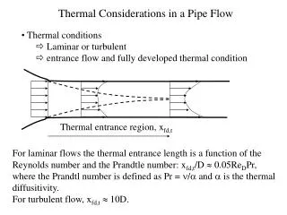
1. Thermal Considerations in a Pipe Flow • Thermal conditions • Laminar or turbulent • entrance flow and fully developed thermal condition Thermal entrance region, xfd,t For laminar flows the thermal entrance length is a function of the Reynolds number and the Prandtle number: xfd,t/D  0.05ReDPr, where the Prandtl number is defined as Pr = / and a is the thermal diffusitivity. For turbulent flow, xfd,t  10D.

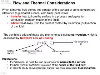
2. h(x) constant x xfd,t Thermal Conditions • For a fully developed pipe flow, the convection coefficient is a constant and is not varied along the pipe length. (as long as all thermal and flow properties are constant also.) • Newton’s law of cooling: q”S = hA(TS-Tm) • Question: since the temperature inside a pipe flow is not constant, what temperature we should use. A mean temperature Tm is defined.

3. Energy Transfer Consider the total thermal energy carried by the fluid as Now image this same amount of energy is carried by a body of fluid with the same mass flow rate but at a uniform mean temperature Tm. Therefore Tm can be defined as Consider Tm as the reference temperature of the fluid so that the total heat transfer between the pipe and the fluid is governed by the Newton’s cooling law as: qs”=h(Ts-Tm), where h is the local convection coefficient, and Ts is the local surface temperature. Note: usually Tm is not a constant and it varies along the pipe depending on the condition of the heat transfer.

4. Energy Balance Example: We would like to designa solar water heater that can heat up the water temperature from 20° C to 50° C at a water flow rate of 0.15 kg/s. The water is flowing through a 5 cm diameter pipe and is receiving a net solar radiation flux of 200 W per unit length (meter). Determine the total pipe length required to achieve the goal.

5. Example (cont.) Questions: (1)How do we determine the heat transfer coefficient, h? There are a total of six parameters involving in this problem:h, V, D, n, kf, cp. The last two variables are thermal conductivity and the specific heat of the water. The temperature dependence is implicit and is only through the variation of thermal properties. Density r is included in the kinematic viscosity, n=m/r. According to the Buckingham theorem, it is possible for us to reduce the number of parameters by three. Therefore, the convection coefficient relationship can be reduced to a function of only three variables: Nu=hD/kf, Nusselt number, Re=VD/n, Reynolds number, and Pr=n/a, Prandtle number. This conclusion is consistent with empirical observation, that is Nu=f(Re, Pr). If we can determine the Reynolds and the Prandtle numbers, we can find the Nusselt number, hence, the heat transfer coefficient, h.

6. Convection Correlations Fixed Re Fixed Pr ln(Nu) ln(Nu) slope m slope n ln(Pr) ln(Re)

7. Empirical Correlations Note: This equation can be used only for moderate temperature difference with all the properties evaluated at Tm. Other more accurate correlation equations can be found in other references. Caution: The ranges of application for these correlations can be quite different.

8. Example (cont.) In our example, we need to first calculate the Reynolds number: water at 35°C, Cp=4.18(kJ/kg.K), m=7x10-4 (N.s/m2), kf=0.626 (W/m.K), Pr=4.8.

9. Energy Balance Question (2): How can we determine the required pipe length? Use energy balance concept: (energy storage) = (energy in) minus (energy out). energy in = energy received during a steady state operation (assume no loss) q’=q/L Tin Tout

10. Temperature Distribution Question (3): Can we determine the water temperature variation along the pipe? Question (4): How about the surface temperature distribution?

11. Temperature variation for constant heat flux Constant temperature difference due to the constant heat flux. Note: These distributions are valid only in the fully developed region. In the entrance region, the convection condition should be different. In general, the entrance length x/D10 for a turbulent pipe flow and is usually negligible as compared to the total pipe length.