Download
1 / 84
840 likes | 1.12k Vues
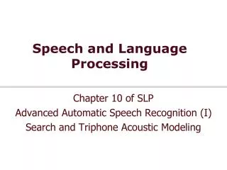
Speech and Language Processing. Chapter 9 of SLP Automatic Speech Recognition (II). Outline for ASR. ASR Architecture The Noisy Channel Model Five easy pieces of an ASR system Language Model Lexicon/Pronunciation Model (HMM) Feature Extraction Acoustic Model Decoder Training

E N D
Speech and Language Processing Chapter 9 of SLP Automatic Speech Recognition (II)
Outline for ASR • ASR Architecture • The Noisy Channel Model • Five easy pieces of an ASR system • Language Model • Lexicon/Pronunciation Model (HMM) • Feature Extraction • Acoustic Model • Decoder • Training • Evaluation Speech and Language Processing Jurafsky and Martin
Acoustic Modeling (= Phone detection) • Given a 39-dimensional vector corresponding to the observation of one frame oi • And given a phone q we want to detect • Compute p(oi|q) • Most popular method: • GMM (Gaussian mixture models) • Other methods • Neural nets, CRFs, SVM, etc Speech and Language Processing Jurafsky and Martin
Problem: how to apply HMM model to continuous observations? • We have assumed that the output alphabet V has a finite number of symbols • But spectral feature vectors are real-valued! • How to deal with real-valued features? • Decoding: Given ot, how to compute P(ot|q) • Learning: How to modify EM to deal with real-valued features Speech and Language Processing Jurafsky and Martin
Vector Quantization • Create a training set of feature vectors • Cluster them into a small number of classes • Represent each class by a discrete symbol • For each class vk, we can compute the probability that it is generated by a given HMM state using Baum-Welch as above Speech and Language Processing Jurafsky and Martin
VQ • We’ll define a • Codebook, which lists for each symbol • A prototype vector, or codeword • If we had 256 classes (‘8-bit VQ’), • A codebook with 256 prototype vectors • Given an incoming feature vector, we compare it to each of the 256 prototype vectors • We pick whichever one is closest (by some ‘distance metric’) • And replace the input vector by the index of this prototype vector Speech and Language Processing Jurafsky and Martin
VQ Speech and Language Processing Jurafsky and Martin
VQ requirements • A distance metric or distortion metric • Specifies how similar two vectors are • Used: • to build clusters • To find prototype vector for cluster • And to compare incoming vector to prototypes • A clustering algorithm • K-means, etc. Speech and Language Processing Jurafsky and Martin
Distance metrics • Simplest: • (square of) Euclidean distance • Also called ‘sum-squared error’ Speech and Language Processing Jurafsky and Martin
Distance metrics • More sophisticated: • (square of) Mahalanobis distance • Assume that each dimension of feature vector has variance 2 • Equation above assumes diagonal covariance matrix; more on this later Speech and Language Processing Jurafsky and Martin
Training a VQ system (generating codebook): K-means clustering 1. Initialization choose M vectors from L training vectors (typically M=2B) as initial code words… random or max. distance. 2. Search: for each training vector, find the closest code word, assign this training vector to that cell 3. Centroid Update: for each cell, compute centroid of that cell. The new code word is the centroid. 4. Repeat (2)-(3) until average distance falls below threshold (or no change) Slide from John-Paul Hosum, OHSU/OGI Speech and Language Processing Jurafsky and Martin
5 0 0 0 1 1 1 2 2 2 3 3 3 4 4 4 5 5 5 6 6 6 7 7 7 8 8 8 9 9 9 0 1 2 3 4 6 7 8 9 Vector Quantization Slide thanks to John-Paul Hosum, OHSU/OGI • Example • Given data points, split into 4 codebook vectors with initial • values at (2,2), (4,6), (6,5), and (8,8) Speech and Language Processing Jurafsky and Martin
5 0 0 0 1 1 1 2 2 2 3 3 3 4 4 4 5 5 5 6 6 6 7 7 7 8 8 8 9 9 9 0 1 2 3 4 6 7 8 9 Vector Quantization Slide from John-Paul Hosum, OHSU/OGI • Example • compute centroids of each codebook, re-compute nearest • neighbor, re-compute centroids... Speech and Language Processing Jurafsky and Martin
6 0 1 2 3 4 5 6 7 8 9 0 1 2 3 4 5 7 8 9 Vector Quantization Slide from John-Paul Hosum, OHSU/OGI • Example • Once there’s no more change, the feature space will bepartitioned into 4 regions. Any input feature can be classified • as belonging to one of the 4 regions. The entire codebook • can be specified by the 4 centroid points. Speech and Language Processing Jurafsky and Martin
Summary: VQ • To compute p(ot|qj) • Compute distance between feature vector ot • and each codeword (prototype vector) • in a preclustered codebook • where distance is either • Euclidean • Mahalanobis • Choose the vector that is the closest to ot • and take its codeword vk • And then look up the likelihood of vk given HMM state j in the B matrix • Bj(ot)=bj(vk) s.t. vk is codeword of closest vector to ot • Using Baum-Welch as above Speech and Language Processing Jurafsky and Martin
Computing bj(vk) feature value 2for state j feature value 1 for state j 14 1 • bj(vk) = number of vectors with codebook index k in state j • number of vectors in state j = = 56 4 Slide from John-Paul Hosum, OHSU/OGI Speech and Language Processing Jurafsky and Martin
Summary: VQ • Training: • Do VQ and then use Baum-Welch to assign probabilities to each symbol • Decoding: • Do VQ and then use the symbol probabilities in decoding Speech and Language Processing Jurafsky and Martin
Directly Modeling Continuous Observations • Gaussians • Univariate Gaussians • Baum-Welch for univariate Gaussians • Multivariate Gaussians • Baum-Welch for multivariate Gausians • Gaussian Mixture Models (GMMs) • Baum-Welch for GMMs Speech and Language Processing Jurafsky and Martin
Better than VQ • VQ is insufficient for real ASR • Instead: Assume the possible values of the observation feature vector ot are normally distributed. • Represent the observation likelihood function bj(ot) as a Gaussian with mean j and variance j2 Speech and Language Processing Jurafsky and Martin
Gaussians are parameters by mean and variance Speech and Language Processing Jurafsky and Martin
Reminder: means and variances • For a discrete random variable X • Mean is the expected value of X • Weighted sum over the values of X • Variance is the squared average deviation from mean Speech and Language Processing Jurafsky and Martin
Gaussian as Probability Density Function Speech and Language Processing Jurafsky and Martin
Gaussian PDFs • A Gaussian is a probability density function; probability is area under curve. • To make it a probability, we constrain area under curve = 1. • BUT… • We will be using “point estimates”; value of Gaussian at point. • Technically these are not probabilities, since a pdf gives a probability over a internvl, needs to be multiplied by dx • As we will see later, this is ok since same value is omitted from all Gaussians, so argmax is still correct. Speech and Language Processing Jurafsky and Martin
Gaussians for Acoustic Modeling • P(o|q): A Gaussian is parameterized by a mean and a variance: Different means P(o|q) is highest here at mean P(o|q is low here, very far from mean) P(o|q) o Speech and Language Processing Jurafsky and Martin
Using a (univariate Gaussian) as an acoustic likelihood estimator • Let’s suppose our observation was a single real-valued feature (instead of 39D vector) • Then if we had learned a Gaussian over the distribution of values of this feature • We could compute the likelihood of any given observation ot as follows: Speech and Language Processing Jurafsky and Martin
Training a Univariate Gaussian • A (single) Gaussian is characterized by a mean and a variance • Imagine that we had some training data in which each state was labeled • We could just compute the mean and variance from the data: Speech and Language Processing Jurafsky and Martin
Training Univariate Gaussians • But we don’t know which observation was produced by which state! • What we want: to assign each observation vector ot to every possible state i, prorated by the probability the the HMM was in state i at time t. • The probability of being in state i at time t is t(i)!! Speech and Language Processing Jurafsky and Martin
Multivariate Gaussians • Instead of a single mean and variance : • Vector of means and covariance matrix Speech and Language Processing Jurafsky and Martin
Multivariate Gaussians • Defining and • So the i-jth element of is: Speech and Language Processing Jurafsky and Martin
Gaussian Intuitions: Size of • = [0 0] = [0 0] = [0 0] • = I = 0.6I = 2I • As becomes larger, Gaussian becomes more spread out; as becomes smaller, Gaussian more compressed Text and figures from Andrew Ng’s lecture notes for CS229 Speech and Language Processing Jurafsky and Martin
From Chen, Picheny et al lecture slides Speech and Language Processing Jurafsky and Martin
[1 0] [.6 0][0 1] [ 0 2] • Different variances in different dimensions Speech and Language Processing Jurafsky and Martin
Gaussian Intuitions: Off-diagonal • As we increase the off-diagonal entries, more correlation between value of x and value of y Text and figures from Andrew Ng’s lecture notes for CS229 Speech and Language Processing Jurafsky and Martin
Gaussian Intuitions: off-diagonal • As we increase the off-diagonal entries, more correlation between value of x and value of y Text and figures from Andrew Ng’s lecture notes for CS229 Speech and Language Processing Jurafsky and Martin
Gaussian Intuitions: off-diagonal and diagonal • Decreasing non-diagonal entries (#1-2) • Increasing variance of one dimension in diagonal (#3) Text and figures from Andrew Ng’s lecture notes for CS229 Speech and Language Processing Jurafsky and Martin
In two dimensions From Chen, Picheny et al lecture slides Speech and Language Processing Jurafsky and Martin
But: assume diagonal covariance • I.e., assume that the features in the feature vector are uncorrelated • This isn’t true for FFT features, but is true for MFCC features, as we will see. • Computation and storage much cheaper if diagonal covariance. • I.e. only diagonal entries are non-zero • Diagonal contains the variance of each dimension ii2 • So this means we consider the variance of each acoustic feature (dimension) separately Speech and Language Processing Jurafsky and Martin
Diagonal covariance • Diagonal contains the variance of each dimension ii2 • So this means we consider the variance of each acoustic feature (dimension) separately Speech and Language Processing Jurafsky and Martin
Baum-Welch reestimation equations for multivariate Gaussians • Natural extension of univariate case, where now i is mean vector for state i: Speech and Language Processing Jurafsky and Martin
But we’re not there yet • Single Gaussian may do a bad job of modeling distribution in any dimension: • Solution: Mixtures of Gaussians Figure from Chen, Picheney et al slides Speech and Language Processing Jurafsky and Martin
Mixtures of Gaussians • M mixtures of Gaussians: • For diagonal covariance: Speech and Language Processing Jurafsky and Martin
GMMs • Summary: each state has a likelihood function parameterized by: • M Mixture weights • M Mean Vectors of dimensionality D • Either • M Covariance Matrices of DxD • Or more likely • M Diagonal Covariance Matrices of DxD • which is equivalent to • M Variance Vectors of dimensionality D Speech and Language Processing Jurafsky and Martin
Where we are • Given: A wave file • Goal: output a string of words • What we know: the acoustic model • How to turn the wavefile into a sequence of acoustic feature vectors, one every 10 ms • If we had a complete phonetic labeling of the training set, we know how to train a gaussian “phone detector” for each phone. • We also know how to represent each word as a sequence of phones • What we knew from Chapter 4: the language model • Next: • Seeing all this back in the context of HMMs • Search: how to combine the language model and the acoustic model to produce a sequence of words Speech and Language Processing Jurafsky and Martin
Decoding • In principle: • In practice: Speech and Language Processing Jurafsky and Martin
Why is ASR decoding hard? Speech and Language Processing Jurafsky and Martin
HMMs for speech Speech and Language Processing Jurafsky and Martin
HMM for digit recognition task Speech and Language Processing Jurafsky and Martin
The Evaluation (forward) problem for speech • The observation sequence O is a series of MFCC vectors • The hidden states W are the phones and words • For a given phone/word string W, our job is to evaluate P(O|W) • Intuition: how likely is the input to have been generated by just that word string W Speech and Language Processing Jurafsky and Martin
Evaluation for speech: Summing over all different paths! • f ay ay ay ay v v v v • f f ay ay ay ay v v v • f f f f ay ay ay ay v • f f ay ay ay ay ay ay v • f f ay ay ay ay ay ay ay ay v • f f ay v v v v v v v Speech and Language Processing Jurafsky and Martin
The forward lattice for “five” Speech and Language Processing Jurafsky and Martin