MACROECONOMICS
1.63k likes | 1.74k Vues
MACROECONOMICS. B. Schmidt Hull College of Business Augusta State University. How I BEGIN Class. Try to make it REAL and PERSONAL to the student Discuss current events Try to make it FUN Encourage opinions Try to increase COMPREHENSION and RETENTION Demand participation.

MACROECONOMICS
E N D
Presentation Transcript
MACROECONOMICS B. Schmidt Hull College of Business Augusta State University
How I BEGIN Class • Try to make it REAL and PERSONAL to the student • Discuss current events • Try to make it FUN • Encourage opinions • Try to increase COMPREHENSION and RETENTION • Demand participation
FIRST things FIRST: • DETERMINE what they know • Correctly Draw and Label the following graphs: S/D, LS/LD, SLF/DLF, AS/AD, MS/MD, PPF, PF
What is the immediate short-term result of the following statement
Various Graphs AS NIR MS PL RGDP Good x PF PPF MD AD Good y MC LS RWR QM RGDP MB LD Labor Loanable Funds Goods & Services Labor P S LS RIR RWR SLF Surplus Market effecting Price Floor shortage, Market effecting Price Ceiling D LD DLF Q Labor LF DurpluD Deficit SLF PSLF RIR RIR RIR PSLF SLF DLF DLF LF LF
PPF & PF Good x RGDP PF Attainable, efficient Unattainable Unattainable Attainable, inefficient Attainable PPF GOOD y Labor
S P P S1 S2 S2 S1 D D Q Q • CURVE SHIFTS: • $ S = #price of Substitute in production • $ S = $price of compliment • $ S = $resource price or other input price • $ S = #price of the good is expected to rise • $ S = $number of sellers • $ S = $productivity
D P P S S D1 D2 D2 D1 Q Q • CURVE SHIFTS: • $ D = $price of substitute in consumption • $ D = #price of compliment • $ D = $price of good is expected to fall • $ D = #price of the good is expected to rise • $ D = $number of sellers • $ D = $productivity
LS WAGE WAGE LS1 LS2 LS2 LS1 LD LD LABOR LABOR • CURVE SHIFTS: • $ LS = #taxes • $ LS = #unemployment • $ LS = $population
LD WAGE WAGE LS LS LD2 LD1 LD1 LD2 LABOR LABOR
MS MS1 MS2 MS2 MS1 NIR NIR MD MD QM QM • CURVE SHIFTS: • $ MS = #RRR • $ MS = #Disc rate • $ MS = Selling Securities
MD MS MS NIR NIR MD2 MD1 MD1 MD2 QM QM • CURVE SHIFTS: • # MD = #PL • # MD = #RGDP • Financial Technology • # MD = #ATMs • $ MD = #Credit Cards
AS PL PL AS1 AS2 AS2 AS1 AD AD RGDP RGDP • CURVE SHIFTS: • # AS = #Pot. GDP • # AS = $MWR • # AS = $Money price of other resource
AD PL PL AS AS AD2 AD1 AD1 AD2 RGDP RGDP • CURVE SHIFTS: • # AD = #Exp. Future income, inflation, profits • # AD = #Govt. Expenditure • # AD = #Global economy (expands) • # AD = #qty money • # AD = $Exchange rate • # AD = $taxes • # AD = $Interest rate
SLF RIR RIR SLF1 SLF2 SLF2 SLF1 DLF DLF LF LF • CURVE SHIFTS: • # SLF = #Disp. income • # SLF = $Wealth • # SLF = $Exp. Future income
DLF RIR RIR SLF SLF DLF2 DLF1 DLF1 DLF2 LF LF • CURVE SHIFTS: • # DLF = #Exp. profit • Bus. Cycle expansion • Technology, successful new products • # Population
SURPLUS WAGE P LS S LABOR SURPLUS SURPLUS LD D LABOR Q
SHORTAGE WAGE P LS S SHORTAGE LABOR SHORTAGE LD D LABOR Q
What is the immediate short-term result of the following statement
Analyzing the News The article points out that there are anomalies such as Belarus and Jamaica where low GDP countries have won a lot of hardware. In the case of Belarus they also point out that its success could be due to the fact that it was a former Soviet bloc country where the Olympics were a substantial focus.
Summary: Key Points in the Article A depression is defined as a severe recession. But what constitutes severe? Since the Great Depression of the 1930s we have had short-lived and relatively shallow downturns in economic activity. But many forecasters and pundits are throwing the term 'depression' around this time. While economic conditions do appear to be dire they are not yet of the same magnitude as the Great Depression. GDP fell 27 percent between 1929 and 1933. In the current downturn we are only down 2.5 to 3 percent. The stock market lost 90 percent of its value in the Great Depression and we are only down 35 to 40 percent now. One third of all banks failed in the Great Depression. And, while the current bank failures are large, they are numbered in the dozens. By any metric we are not in a depression. However, the period leading up to the Great Depression has some similarities that are alarming. A period of prosperity in the 1920s led to asset price bubbles and a faltering banking system. However, the current belief is that we learned from our policy mistakes of the 1930s. The Fed has been aggressive in addressing the liquidity crisis. In addition the government appears to be near additional massive fiscal stimulus. Only time will tell whether we have better tools today to keep this downturn classified as a recession.
Analyzing the News Where are we on the business cycle? Unfortunately we won't know until later. Did the aggressive monetary and fiscal stimulus work? I'll let you know in a few years but until then we will all be speculating. Was it enough? Was it too much? Will it get better or worse? It appears we have not been able to prevent downturns nor predict their magnitude. Economic intervention is still more art than science.
Guns Versus Butter The figure shows the change in the quantity of defense goods and services produced. It increases in times of war and decreases in times of peace.
Guns Versus Butter During the 1990s, U.S. production possibilities were shown by PPF0. President Reagan raised the stakes in the Cold War and the United States was producing at point A. By mid-1990s, the United States enjoyed a peace dividend and production moved to point B.
Guns Versus Butter During the next decade, production possibilities expanded to PPF1. The United States could have kept defense production constant and moved to point C. But after 9/11, defense production increased and the United States moved to point D.
Hong Kong’s Rapid Economic Growth • In 1960, Hong Kong’s production possibilities were25 percent of those in the United States. • In 1960, the United States and Hong Kong produced at point A on their respective PPFs.
Hong Kong’s Rapid Economic Growth • Hong Kong allocated more resources to producing capital goods than the United States did. • And by 2008, Hong Kong’s PPF was 80 percent of U.S. PPF.
Hong Kong’s Rapid Economic Growth • If Hong Kong continues to produce at a point like B, allocating more resources to producing capital goods, it will grow more rapidly than the United States.
Hong Kong’s Rapid Economic Growth • But if Hong Kong produces at a point like D, its economic growth rate will slow.
Business cycle What cycle are we currently in?
13.1 BUSINESS-CYCLE DEFINITIONS AND FACTS • U.S. Business-Cycle History • The NBER has identified 33 complete cycles starting from a trough in December 1854. • Over all 33 complete cycles: • The average length of an expansion is 35 months and the average length of a recession is 18 months. • The average time from trough to trough is 53 months.
13.1 BUSINESS-CYCLE DEFINITIONS AND FACTS • So over the 152 years since 1854, the U.S. economy has been in: • Recession for about one third of the time • Expansion for about two thirds of the time. • The 152-year averages hide significant changes that have occurred in the length of a cycle and the relative length of the recession and expansion phases.
13.1 BUSINESS-CYCLE DEFINITIONS AND FACTS Figure 13.1 summarizes U.S. recession, expansion, and cycle length since 1854. Recessions have shortened. Expansions have lengthened, and complete cycles have lengthened.
The National Bureau Calls a Recession • The NBER’s Business Cycle Dating Committee announced in November 2001 that a peak in business activity has occurred in the U.S. economy in March 2001. • To identify the date of the cycle peak, the NBER committee looked at industrial production, employment, real income, and wholesale and retail sales. • The figure on the next slide shows employment.
The National Bureau Calls a Recession • Employment peaked in March 2001. • Other factors considered by the committee did not peak but didn't contradict the employment numbers. • So the committee was clear that March was the peak month.
TheNationalBureau Calls a Recession • The NBER committee gives relatively little weight to real GDP. • The figure shows that through 2000, real GDP exceeded potential GDP. • Real GDP was shrinking during the first quarter of 2001, before the NBER says the recession began.
TheNationalBureau Calls a Recession • In July 2003, the NBER committee announced that a new expansion had begun in November 2001. • The figure shows that this timing lined up better with real GDP than with employment.
TheNational Bureau Calls a Recession • The employment trough didn’t occur until April 2002. • This lagging of employment behind real GDP is normal and occurs in all expansions.
The Global Business Cycle • Every economy has a business cycle, but they differ in severity and timing. • The U.S. cycle in the early 1908s was the most severe. • The U.S. cycle leads the cycle in Europe and Japan. • Japan’s cycle has taken a downward trend since early 1990s.
The Global Business Cycle • The figure shows the business cycle in the world economy. • The figure shows no recession in the world as a whole since 1980. • and that the Asian economies are driving the world economy.
Oil Price Cycles in the U.S. and Global Economies • In September 1973, OPEC cut production and raised the price of crude oil to $10 a barrel—$30 in 2000 dollars. • In United States, Europe, Japan and developed nations went into recession.
Oil Price Cycles in the U.S. and Global Economies • In 1980, OPEC again cut production and raised the price to $37 a barrel—almost $70 in 2000 dollars. • The global economy experienced recession, but more severe than the mid-1970 one because the Fed’s monetary policy cut aggregate demand.
Oil Price Cycles in the U.S. and Global Economies • With the price of crude oil so high, Canada and the United States increased production. • Britain and Norway developed North Sea oil and Mexico stepped up production. • The price tumbled.
Oil Price Cycles in the U.S. and Global Economies • Strong Asian demand for oil increased its price in the 2000s. • By 2007, the price has surged to almost $60 a barrel. • By the summer of 2008, the price was $145 a barrel.
Real GDP Growth, Inflation, and the Business Cycle • Each dot represents a year between 1970 and 2007. • Dots move rightward, which shows economic growth. • Dots move upward, which shows inflation.
Real GDP Growth, Inflation, and the Business Cycle • The dots move in waves, which show the business cycle and the recessions. • Sometimes the economy is at full employment as it was in 1970. • Sometimes there is an output gap as in 2007.