Download
1 / 11
110 likes | 267 Vues
Commentary on Time Series in High Energy Astrophysics. Brandon C. Kelly Harvard-Smithsonian Center for Astrophysics. Trends. Lightcurve shape determined by time and parameters Examples: SNe , γ -ray bursts Can use parameteric methods to characterize shape

E N D
Commentary on Time Series in High Energy Astrophysics Brandon C. Kelly Harvard-Smithsonian Center for Astrophysics
Trends • Lightcurve shape determined by time and parameters • Examples: SNe, γ-ray bursts • Can use parameteric methods to characterize shape • E.g., Rise and decay time scale of a pulse • Can use non-parameteric methods to characterize shape • Joey: Projected spline fits of LC onto diffusion map space • Ashish: Used dm/dt to obtain simple parameterization of trends for sparse LC Spline fits to SNeLCs in multiple bands (Richards+, 2011)
Periodic Behavior • LC shape determined by time and parameters, repeats regularly • Examples: Eclipsing binaries, Pulsars • Characterized by period, shape of pulse • Pavlos: Described methods for estimating periods in noisy and irregularly sampled time series • Eric: Use H-test on photon arrival times to find periods, regularly sampled time series Pulsar Eclipsing Binary Credit: ESA
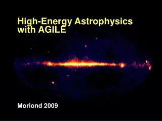
Stochastic Variations Cygnus X-1 • Stochastic Process: LC depends stochastically on previous values of LC and time between observations • Examples: Random-walk behavior, accretion flows, jets • Joey: Used parameters that summarize stochastic fluctuations for classification Radio X-ray Wilms+ (2007)
Characterizing Stochastic Processes Mrk 766, Vaughan & Fabian (2003) What similarities exist between these two segments?
How to quantify features of stochastic processes? Compare to More variable on long timescales More variable on short timescales Compare to Lower Variability Higher Variability
Characterizing Variability of Stochastic Processes • Use features in the autocorrelation function (ACF) and power spectral density (PSD) • ACF: Correlation of variations in time series as a function of Δt • PSD: Variability power per frequency interval • ACF and PSD are Fourier transforms of each other (modulo a normalization factor) • Weak Stationarity: Mean and ACF of do not change with time Variability power concentrated on longer time scales Variability power concentrated on shorter time scales
Parameteric Modeling of Stochastic Processes • Non-parameteric methods (e.g., periodogram) require high-quality data • No Assumptions about functional form of PSD or ACF • Noisy • Suffer biases from sampling pattern • Parameteric modeling of PSD possible through monte-carlo methods (e.g., Uttley+ 2002) • Can fit arbitrary PSDs for any sampling pattern • Computationally expensive • Not most efficient use of information in data • Parameteric modeling in time domain • Use a parameteric model for time-evolution of stochastic process • Fitting is done via maximum-likelihood or Bayesian methods • Computationally cheap for many models
Example: Ornstein-Uhlenbeck Process (i.e., Damped Random Walk) • AGN optical and X-ray LCs well described by one or more OU processes (Kelly+2009,2011, MacLeod+2010): • Likelihood function derived from solution PSD Frequency Time, MacLeod+ 2010 Time, Kelly+ 2011
Classifying Variable Sources • Use the various variability metrics (parameters) for classification • Classification of variables (Joey): • Improve source selection/classification based on color and other quantities • Find new classes of objects • Identification of short-lived (transient) phenomena (Ashish) • Time-sensitive, so classification must be done in real time with sparse time series • Can use variability + other info to identify best strategy for follow-up observations (Joey, Ashish)
Directions for Future Work • Improve modeling of stochastic processes in time-domain (e.g., through Stoch. Diff. Eq.) • Incorporate multi-wavelength correlations, lags • Include stochastic flaring activity • Develop time-domain models for arbitrary PSDs • Improved computational methods/strategies (Eric) • Future massive data sets will either require efficient programs and efficient use of memory or analyzing a subset of the data • Improvement in handling of differences between training and test sets for classification (Joey)