Review
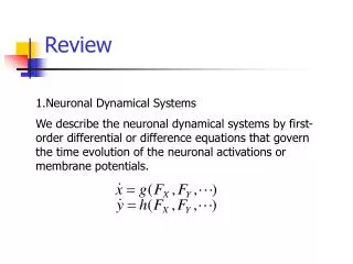
Review. 1.Neuronal Dynamical Systems. We describe the neuronal dynamical systems by first-order differential or difference equations that govern the time evolution of the neuronal activations or membrane potentials. Review. 4.Additive activation models. Hopfield circuit:.

Review
E N D
Presentation Transcript
Review 1.Neuronal Dynamical Systems We describe the neuronal dynamical systems by first-order differential or difference equations that govern the time evolution of the neuronal activations or membrane potentials.
Review 4.Additive activation models Hopfield circuit: • Additive autoassociative model; • Strictly increasing bounded signal function ; • Synaptic connection matrix is symmetric .
Review 5.Additive bivalent models Lyapunov Functions Cannot find a lyapunov function,nothing follows; Can find a lyapunov function,stability holds.
Review A dynamics system is stable , if ; asymptotically stable, if . Monotonicity of a lyapunov function is a sufficient not necessary condition for stability and asymptotic stability.
Review Bivalent BAM theorem. Every matrix is bidirectionally stable for synchronous or asynchronous state changes. • Synchronous:update an entire field of neurons at a time. • Simple asynchronous:only one neuron makes a state-change decision. • Subset asynchronous:one subset of neurons per field makes state-change decisions at a time.
Chapter 3. Neural Dynamics II:Activation Models The most popular method for constructing M:the bipolar Hebbian or outer-product learning method binary vector associations: bipolar vector associations:
Chapter 3. Neural Dynamics II:Activation Models The binary outer-product law: The bipolar outer-product law: The Boolean outer-product law:
Chapter 3. Neural Dynamics II:Activation Models The weighted outer-product law: Where holds. In matrix notation: Where
Chapter 3. Neural Dynamics II:Activation Models One can models the inherent exponential fading of unsupervised learning laws by rearrange coefficients of the matrix W. Such as , an exponential fading memory, constrained by , results if
Chapter 3. Neural Dynamics II:Activation Models 1.Unweighted encoding skews memory-capacity analyses. 2. The neural-network literature has largely overlooked the weighted outerproduct laws.
Chapter 3. Neural Dynamics II:Activation Models ※ Optimal Linear Associative Memory Matrices Optimal linear associative memory matrices: The pseudo-inverse matrix of : If x is a nonzero scalar: If x is a nonzero vector: If x is a zero scalar or zero vector : For a rectangular matrix , if exists:
Chapter 3. Neural Dynamics II:Activation Models ※ Optimal Linear Associative Memory Matrices Define the matrix Euclidean norm as Minimize the mean-squared error of forward recall,to find that satisfies the relation
Chapter 3. Neural Dynamics II:Activation Models ※ Optimal Linear Associative Memory Matrices Suppose further that the inverse matrix exists. Then So the OLAM matrix correspond to
Chapter 3. Neural Dynamics II:Activation Models If the set of vector is orthonormal Then the OLAM matrix reduces to the classical linear associative memory(LAM) : For is orthonormal, the inverse of is .
Chapter 3. Neural Dynamics II:Activation Models ※ Autoassociative OLAM Filtering Autoassociative OLAM systems behave as linear filters. In the autoassociative case the OLAM matrix encodes only the known signal vectors . Then the OLAM matrix equation (3-78) reduces to M linearly “filters” input measurement x to the output vector by vector matrix multiplication: .
Chapter 3. Neural Dynamics II:Activation Models ※3.6.2 Autoassociative OLAM Filtering The OLAM matrix behaves as a projection operator. Algebraically,this means the matrix M is idempotent: . Since matrix multiplication is associative,pseudo-inverse property (3-80) implies idempotency of the autoassociative OLAM matrix
Chapter 3. Neural Dynamics II:Activation Models ※ Autoassociative OLAM Filtering Then (3-80) also implies that the additive dual matrix behaves as a projection operator: We can represent a projection matrix M as the mapping
Chapter 3. Neural Dynamics II:Activation Models ※ Autoassociative OLAM Filtering The Pythagorean theorem underlies projection operators. The known signal vectors span some unique linear subspace of L equals , the set of all linear combinations of the m known signal vectors. denotes the orthogonal complement space the set of all real n-vectors x orthogonal to every n-vector y in L.
Chapter 3. Neural Dynamics II:Activation Models ※ Autoassociative OLAM Filtering • Operator projects onto L. • The dual operator projects onto . Projection Operator and uniquely decompose every vector x into a summed signal vector and a noise or novelty vector : x
Chapter 3. Neural Dynamics II:Activation Models ※ Autoassociative OLAM Filtering The unique additive decomposition obeys a generalized Pythagorean theorem: where defines the squared Euclidean or norm. Kohonen[1988] calls the novelty filter on .
Chapter 3. Neural Dynamics II:Activation Models ※ Autoassociative OLAM Filtering Projection measures what we know about input x relative to stored signal vectors : for some constant vector . The novelty vector measures what is maximally unknown or novel in the measured input signal x.
Chapter 3. Neural Dynamics II:Activation Models ※Autoassociative OLAM Filtering Suppose we model a random measurement vector x as a random signal vector corrupted by an additive, independent random-noise vector : We can estimate the unknown signal as the OLAM-filtered output .
Chapter 3. Neural Dynamics II:Activation Models ※Autoassociative OLAM Filtering Kohonen[1988] has shown that if the multivariable noise distribution is radially symmetric, such as a multivariable Gaussian distribution,then the OLAM capacity m and pattern dimension n scale the variance of the random-variable estimator-error norm :
Chapter 3. Neural Dynamics II:Activation Models ※Autoassociative OLAM Filtering 1.The autoassociative OLAM filter suppress noise if m<n , when memory capacity does not exceed signal dimension. 2.The OLAM filter amplifies noise if m>n, when capacity exceeds dimension.
Chapter 3. Neural Dynamics II:Activation Models ※BAM Correlation Encoding Example The above data-dependent encoding schemes add outer-product correlation matrices. The following example illustrates a complete nonlinear feedback neural network in action,with data deliberately encoded into the system dynamics.
Chapter 3. Neural Dynamics II:Activation Models ※BAM Correlation Encoding Example Suppose the data consists of two unweighted binary associations and defined by the nonorthogonal binary signal vectors:
Chapter 3. Neural Dynamics II:Activation Models ※BAM Correlation Encoding Example These binary associations correspond to the two bipolar associations and defined by the bipol –ar signal vectors:
Chapter 3. Neural Dynamics II:Activation Models ※BAM Correlation Encoding Example We compute the BAM memory matrix M by adding the bipol –ar correlation matrices and pointwise. The first correlation matrix equals
Chapter 3. Neural Dynamics II:Activation Models ※BAM Correlation Encoding Example Observe that the i th row of the correlation matrix equals the bipolar vector multipled by the i th element of . The j th column has the similar result. So equals
Chapter 3. Neural Dynamics II:Activation Models ※BAM Correlation Encoding Example Adding these matrices pairwise gives M:
Chapter 3. Neural Dynamics II:Activation Models ※BAM Correlation Encoding Example Suppose, first,we use binary state vectors.All update policies are synchronous.Suppose we present binary vector as input to the system—as the current signal state vector at . Then applying the threshold law (3-26) synchronously gives
Chapter 3. Neural Dynamics II:Activation Models ※BAM Correlation Encoding Example Passing through the backward filter , and applying the bipolar version of the threshold law(3-27),gives back : So is a fixed point of the BAM dynamical system. It has Lyapunov “energy” , which equals the backward value . has the similar result:a fixed point with energy .
Chapter 3. Neural Dynamics II:Activation Models ※BAM Correlation Encoding Example So the two deliberately encoded fixed points reside in equally “deep”attractors. Hamming distance H equals distance. counts the number of slots in which binary vectors and differ:
Chapter 3. Neural Dynamics II:Activation Models ※BAM Correlation Encoding Example Consider for example the input , which differs from by 1 bit , or . Then
Chapter 3. Neural Dynamics II:Activation Models ※BAM Correlation Encoding Example On average, bipolar signal state vector produce more accurate recall than binary signal state vectors when we use bipolar out-product encoding. Intuitively,binary signal implicitly favor 1s over 0s,wheres bipolarsignals are not biased in favor of 1s or –1s: 1+0=1,whereas 1+(-1)=0
Chapter 3. Neural Dynamics II:Activation Models ※BAM Correlation Encoding Example The nueron do not know that a globle pattern “error” has occurred. They do not know that they should correct the error, or whether their current behavior helps correct it.The network also does not provide the nuerons with a globle error signal, and also Lyapunov “energy” information, though state-changing nuerons decrease the energy. Insteadly, the system dynamics guide the local behavior to a globle reconstruction(recollection) of a learned pattern.
Chapter 3. Neural Dynamics II:Activation Models ※Memory Capacity:Dimensionality Limits Capacity Synaptic connection matrices encode limited information. We sum more correlation matrices ,then holds more frequently. After a point,adding additional associations Does not significantly change the connection matrix. The system “forgets”some patterns. This limits the memory capacity.
Chapter 3. Neural Dynamics II:Activation Models ※Memory Capacity:Dimensionality Limits Capacity Synaptic connection matrices encode limited information. We sum more correlation matrices ,then holds more frequently. After a point,adding additional associations Does not significantly change the connection matrix. The system “forgets”some patterns. This limits the memory capacity.
Chapter 3. Neural Dynamics II:Activation Models ※Memory Capacity:Dimensionality Limits Capacity A general property of nueral network: Dimensionality limits capacity
Chapter 3. Neural Dynamics II:Activation Models ※3.6.4 Memory Capacity:Dimensionality Limits Capacity Grossberg’s sparse coding theorem says , for deterministic encoding ,that pattern dimensionality must exceed pattern number to prevent learning some patterns at the expense of forgetting others. For example,capacity bound for bipolar correlation encoding in the Amari-Hopfield network is
Chapter 3. Neural Dynamics II:Activation Models ※3.6.4 Memory Capacity:Dimensionality Limits Capacity For Boolean encoding of binary associations, the memory capacity of bivalent additive BAMs can greatly exceed min(n,p) to the new upper bound min(2n,2p), if the thresholds Ui and Vj are judiciously choosed. And different sets of thresholds should also improve capacity in the bipolar case(incloding bipolar Hebbian encoding)
Chapter 3. Neural Dynamics II:Activation Models ※The Hopfield Model The Hopfield model illustrates an autoassociative additive bivalent BAM operated serially with simple asynchronous state changes. Autoassociativity means the network topology reduces to only one field, ,of neurons: .The synaptic connection matrix M symmetrically intraconnects the n neurons in field
Chapter 3. Neural Dynamics II:Activation Models ※The Hopfield Model The autoassociative version of Equation (3-24) describes the additive neuronal activation dynamics: (3-87) for constant input , with threshold signal function (3-88)
Chapter 3. Neural Dynamics II:Activation Models ※The Hopfield Model We precompute the Hebbian synaptic connection matrix M by summing bipolar outer-product(autocorrelation)matrices and zeroing the main diagonal: (3-89) where I denotes the n-by-n identity matrix . Zeroing the main diagonal tends to improve recall accuracy by helping the system transfer function behave less like the identity operator.
Chapter 3. Neural Dynamics II:Activation Models ※Additive dynamics and the noise-saturation dilemma Grossberg’s Saturation theorem states that additive activation models saturate for large inputs, but multiplicative models do not .
Chapter 3. Neural Dynamics II:Activation Models Grossberg’s Saturation Theorem The stationary “reflectance pattern” confronts the system amid the background illumination The i th neuron receives input .Convex coefficient defines the “reflectance” : : the passive decay rate : the activation bound
Chapter 3. Neural Dynamics II:Activation Models Additive Grossberg model: We can solve the linear differential equation to yield For initial condition , as time increases the activation converges to its steady-state value: As
Chapter 3. Neural Dynamics II:Activation Models So the additive model saturates. Multiplicative activation model:
Chapter 3. Neural Dynamics II:Activation Models For initial condition ,the solution to this differential equation becomes As time increases, the neuron reaches steady state exponentially fast: (3-96) as .
Chapter 3. Neural Dynamics II:Activation Models This proves the Grossberg saturation theorem: Additive models saturate , multiplicative models do not.

