Download
1 / 11
110 likes | 281 Vues
Coherent Coincident Analysis of LIGO Burst Candidates. Laura Cadonati Massachusetts Institute of Technology LIGO Scientific Collaboration 8 th Gravitational Wave Data Analysis Workshop Milwaukee, Wisconsin, December 17-20, 2003. Post Coincidence Coherent Analysis.

E N D
Coherent Coincident Analysis of LIGO Burst Candidates Laura Cadonati Massachusetts Institute of Technology LIGO Scientific Collaboration 8th Gravitational Wave Data Analysis Workshop Milwaukee, Wisconsin, December 17-20, 2003
Post Coincidence Coherent Analysis • Burst candidates separately identified in the data stream of each interferometer by the Event Trigger Generators (ETG): TFclusters, Excess Power, WaveBurst, BlockNormal. • Tuning maximizes detection efficiency for given classes of waveforms and a given false rate ~ 1-2 Hz • Multi-interferometer coincidence analysis: • Rule of thumb: detection efficiency in coincidence ~ product of efficiency at the single interferometers. Coincidence selection criteria should not further reduce the detection efficiency. The final false rate limits how loose the cuts can be. • Currently implemented: time and frequency coincidence (in general, different tolerance for different trigger generators). • Amplitude/energy cut: not yet implemented. • Cross-Correlation for coherent analysis of coincident events • This is a waveform consistency test. • Allows suppression of false events without reducing the detection efficiency of the pipeline.
Dt = + 10 ms Dt = - 10 ms confidence versus lag 15 Max confidence: CM(t0) = 13.2 at lag = - 0.7 ms 10 confidence 5 0 -10 0 10 lag [ms] r-statistic Cross Correlation Test For each triple coincidence candidate event produced by the burst pipeline (start time, duration DT) process pairs of interferometers: simulated signal, SNR~60, S2 noise Data Conditioning: » 100-2048 Hz band-pass »Whitening with linear error predictor filters Partition the trigger in sub-intervals (50% overlap) of duration t = integration window (20, 50, 100 ms). For each sub-interval, time shift up to 10 ms and build an r-statistic series distribution. If the distribution of the r-statistic is inconsistent with the no-correlation hypothesis: find the time shift yielding maximum correlation confidence CM(j) (j=index for the sub-interval)
CM(j) plots G12 =max(CM12) • Each point: max confidence CM(j) for an interval twide(here: t = 20ms) • Threshold on G: • 2 interferometers: • G=maxj(CM(j) ) > b2 • 3 interferometers: • G=maxj(CM12+ CM13+ CM23)/3 > b3 • In general, we can have b2 b3 • b3=3: 99.9% correlation probability • in each sub-interval G13 =max(CM13) G23 =max(CM23) G=max(CM12 +CM13+CM23)/3 Testing 3 integration windows: 20ms (G20) 50ms (G50) 100ms (G100) in OR: G=max(G20,G50,G100)
SNR definition for excess-power techniques in the burst search = SNRmatched filtering / √2 Triple Coincidence Performance Analysis in S2 • Exploring the test performance for triple coincidence detection, independently from • trigger generators and from previous portions of the analysis pipeline: • Add simulated events to real noise at random times in the 3 LIGO interferometers, • covering 10% of the S2 dataset (in LIGO jargon: triple coincidence playground) • apply r-statistic test to 200 ms around the simulation peak time Definition of quantities used to characterize a burst signal: Total energy in the burst (units: strain/rtHz) [directly comparable to sensitivity curves] For narrow-band bursts with central frequency fc Sh(f)=single-sided reference noise in the S2 Science Run reference S2 SNR for a given amplitude/waveform
(fchar, hrss) [strain/rtHz] with 50% triple coincidence detection probability LHO-4km SNR: SNR > 30 LHO-2km LLO-4km ~ √2|h(f)| [strain/Hz] Detection Efficiency for Narrow-Band Bursts Sine-Gaussian waveform f0=254Hz Q=9 linear polarization, source at zenith Triple coincidence efficiency curve 50% triple coincidence detection probability: hpeak = 3.2e-20 [strain] hrss = 2.3e-21 [strain/rtHz] SNR: LLO-4km=8 LHO-4km=4LHO-2km=3
~ √2|h(f)| [strain/Hz] Detection Efficiency for Broad-Band Bursts Gaussian waveform t=1ms linear polarization, source at zenith (fchar, hrss) [strain/rtHz] with 50% triple coincidence detection probability LHO-4km LHO-2km SNR: LLO-4km SNR > 30 50% triple coincidence detection probability: hpeak = 1.6e-19 [strain] hrss = 5.7e-21 [strain/rtHz] SNR: LLO-4km=11.5 LHO-4km=6LHO-2km=5
R.O.C. Receiver-Operator Characteristics Detection Probability versus False Alarm Probability. Parameter: triple coincidence confidence threshold b3 Simulated 1730 events at fixed hpeak ,hrss (10 events uniformly distributed in each S2 “playground” segment) Tested cross correlation over 200 ms around the peak time Operating condition: b3=3 chosen from first principles (99.9% correlation probability in each event sub-interval for a pair of interferometers), corresponds to a ~1% false alarm probability for triple coincidence events with duration 200 ms.
Trigger numerology “Loose” coincidence cuts coincidence triple coincident clusters (Dt = 30 ms) after frequency cut (200Hz tolerance) after r-statistic test (β3 = 3) Rejection efficiency L1-H1-H2 20 mHz 15 mHz 0.1 mHz (99.35 ± 0.08)% “Tight” coincidence cuts coincidence triple coincident clusters (Dt = 15 ms) after frequency cut (75Hz tolerance) after r-statistic test (β3 = 3) Rejection efficiency L1-H1-H2 6 mHz 1 mHz 0.01 mHz (1/day) (98.8 ± 0.4)% Suppression of Accidental Coincidences from the Pipeline In general: depends on the Event Trigger Generator and the nature of its triggers. In particular: typical distribution of event duration (larger events have more integration windows). Shown here: TFCLUSTERS 130 - 400 Hz (presented in Sylvestre’s talk) Coincident numbers reported here are averages of 6 background measurements: LLO-LHO = ± 8, ± 6, ± 4 sec (H1-H2 together) PRELIMINARY!!
False Probability versus Threshold Histogram of G= max (G20, G50, G100) In general: depends on the trigger generators and the previous portion of the analysis pipeline (typical event duration, how stringent are the selection and coincidence cuts) Shown here: TFCLUSTERS 130-400 Hz with “loose” coincidence cuts G False Probability versus threshold (G>b3) b3=3 0.65% Fraction of surviving events b3
Conclusions • The LIGO burst S1 analysis exclusively relied on event trigger generators and time/frequency coincidences. • The search in the second science run (S2) includes a new module of coherent analysis, added at the end of the burst pipeline: r-statistic test for cross correlation in time domain • Assigns a confidence to coincidence events at the end of the burst pipeline • Verifies the waveforms are consistent • Suppresses false rate in the burst analysis, allowing lower thresholds • Tests of the method, using simulated signals on top of real noise, yield 50% triple coincidence detection efficiency for narrow-band and broad-band bursts at SNR=3-5 in the least sensitive detector (LHO-2km) with a false probability ~1%. • Currently measuring global efficiency and false rate for the S2 pipeline (event analysis + coherent analysis).