Frag statistics for FIA
Frag statistics for FIA. Fragmentation statistics for FIA. Tonya Lister Michael Hoppus. Rachel Riemann Andy Lister Tonya Lister Michael Hoppus. NE-FIA, Northeastern Research Station 11 Campus Blvd, Newtown Square, PA 19073. Because our current statistics don’t tell the whole story….

Frag statistics for FIA
E N D
Presentation Transcript
Frag statistics for FIA Fragmentation statistics for FIA Tonya Lister Michael Hoppus Rachel Riemann Andy Lister Tonya Lister Michael Hoppus NE-FIA, Northeastern Research Station 11 Campus Blvd, Newtown Square, PA 19073
Because our current statistics don’t tell the whole story… Why are we interested in frag? 2 areas of roughly equal %forest (61 and 62%), but different spatial distributions of forest, and/or different contexts (ag vs. residential) that are not captured in the single % number…
Why is FIA interested in frag? We know how much forest there is in an area (e.g. county or watershed) -- ---but how it is distributed? • In what size patches? (and what proportion of it is still part of the forest matrix?) • How isolated or connected are the patches? • How much of it is interior area? And how much of it is in edge conditions? • What is the landuse composition of the surrounding nonforest area?
This information can give us a substantially different picture of the forest resource… Norfolk county– from NLCD’92 dataset -- 55720 ha forest (54% of total land area) 30376 ha interior forest (30% of total land area)
Frag does exist and is of considerable interest… Fragmentation of forestland has been reported in individual studies and discussed as an issue in dedicated conferences and forums in the: • Virginia, • South, • Rocky Mountains, • to name but a few… • Chesapeake, • NY-NJ highlands • Lake States, • Northeast, Bringing up issues related to resource management, landuse planning, health and sustainability… And including considerable interest in having information that is consistent over broad areas to allow for monitoring of frag and landscape change
…and it is continuing to change… --as agriculture and abandoned land are converting back to forest (though this trend is pretty much coming to an end in the northeast) --as continuing development converts more previously forested land--spreading out from urban centers and suburban satellite areas, and new pockets in rural areas --as a regulations and incentive policies are implemented that affect the locations, directions and patterns of landuse development 1949 1979 1998
Frag has an effect on: • Wildlife – species abundance, diversity, breeding success • Forest composition and health – # of exotics, mortality, composition changes • Water quality – flow and flow variability, increased sedimentation, biogeochemical cycles, macroinvertebrates, heavy metal enrichment, • Forest management for timber production – economic sustainability of private industry, treatment constraints • Other – recreation, microclimate… • in general, landscape-level characteristics (such as frag and context) have been observed to be important explanatory ecological variables..
Frag measures found to be correlated to such changes: • Wildlife – patch size, interior area, isolation distance, total amount of forest in surrounding area • Forest composition and health – patch size, amount of edge, distance from edge, proximity to human populations • Water quality – % developed landuses in the watershed, spatial distribution of those landuses, streamside landuse, amount of impervious surface, largest developed patch size • Forest management for timber production – patch size, adjacent landuses • Other – patch size
Having information regarding fragmentation would add substantially to our own interpretation/understanding/reporting of the forest from FIA data. • How fragmented is that forest becoming? • How much of that forestland is still economically viable for timber production? • How much of that forest is still a source for wildlife populations? • How much is under additional health and change pressures because of extensive surrounding development? • How much is still available for recreation?
What is FIA’s role… • At the very least: • We are interested in measuring frag-related info and indices that we can use to better understand, interpret and report the statistics associated with the FIA inventory, • We are interested in monitoring the distribution and fragmentation characteristics of the forest over time, just as we monitor the status and changes in forest area, volume, relative species compositions, etc. • Providing information that is basic and consistent over broad areas • Integrating with information at other scales…
So, what stats/indices should we calculate? • Criteria: • Indices that cover the spectrum of characteristics we are interested in • Indices that are not unnecessarily redundant • Concentrate on simple/basic measures vs. compound complex ones • to avoid combining several factors that may interact • to enhance understandability of what summaries of the values mean • Indices that are related to real changes observed • Indices that don’t have special implementation problems • Indices that are ideally robust to different resolutions of data sources– i.e. changes that may occur when comparing statistics calculated over time…
We chose these types of metrics • % cover (of forest and other landuses) --landscape scale factors continually show up as important and can even override local factors in their apparent impact on water quality, wildlife success, etc. • Distribution/configuration of the forest – e.g. patch sizes continue to appear in the literature as being linked to many of the changes observed with plant and animal species; patch sizes also directly affect the economic feasibility of • Edge – edges between different landuses also continue to show up as places where forest/nonforest interactions are occurring
Calculated for each watershed/region • Percent cover • Forest area (% of total) • Core forest area (%) – can be calculated with and without road • % of each landuse • Distribution/configuration of the forest land • Patch area (frequency distribution) • Patch isolation (nearest neighbor distance, aggregation index) (frequency distribution) • Patch shape (area:perimeter or long:short axis ratios) (frequency distribution) • Edge and adjacent landuses • total perimeter distance and % of each landuse
Calculated for a patch • Status • Patch area • Core area (with and without roads) • Patch isolation (nearest neighbor distance) • A shape index (e.g. perimeter:area) • Edge • Adjacent landuses (total perimeter distance and % of each landuse) • Time • E.g. encapsulation date (I.e. – how long has it been a fragment of this size…)
Calculated for a point/pixel (e.g. FIA plot) • Distance from the nearest edge • Adjacent landuse at that edge • Calculated… • core/edge status • patch/matrix status
Over several scales… • Total forest area (%) • Core forest area (%) – can be calculated with and without road • % of each landuse • Adjacent landuses (% of total edge) and total edge • (e.g. around a plot or patch centroid or stream monitoring site…) • (e.g. 5, 10, 20, 50, 100, 500, 1000, 5000, 10000, 50000 acres…)
the Scale of observation… • There are several instances in which the scale/window of the context data being provided is an important consideration. Acres (radius) 50 | 250m 92% forest For example, in this window, it appears that the surrounding land area is entirely forested.
the Scale of calculation… 80% forest 13% residential 2% agriculture Acres (radius) 500 | 800m • In this window, it appears that the area is primarily forested, with a strip of residential and a few agricultural pixels within the forest matrix
Scale… 59% forest 28% residential 1% ag 2% urban Acres (radius) 5000 | 2.5 km • If we look at the area with a larger window, the forest is now down to about 60% of the area, with residential becoming a substantial component, along with some agricultural and other urban land uses
Scale… 47% forest 33% residential 3% ag 12% urban Acres (radius) 50,000 | 8 km • Taking a larger picture still, residential and other urban landuses now make up as much of the total land area as forest.
Scale… If we isolate our information to just one window size, we will be ignorant of a substantial amount of context information. It is frequently important to have information at several scales in order to determine the trends or thresholds of the impacts/changes observed.
So, given what metrics we’d like,what source data are there… Visual interpretation of very high resolution imagery like aerial photography… or lulc classifications derived from TM Any metrics we calculate DEPEND upon on the accuracy of the source data we’re calculating from:
Advantages of “photo”-derived: • relates more directly to the scale of factors of interest on the ground • relates to individual plots very well (if plots are used as the sample points) advantages… • Advantages of TM-derived: • providescontinuous information • and thus may provide better area statistics • easier to recalculate new indices on the data (photointerp would almost certainly require shortcuts, such as limiting the area being interpreted, limiting the variables being interpreted, etc.) • more chance of getting it at the dates we need
But TM-derived datasets have their own set of challenges 3 datasets of approximately equal per-pixel accuracy (~ 80%), but they appear to be very different in how they depict forest fragmentation. This is affected by the accuracy of the classification (e.g. are residential with trees classed as residential or forest; what are mixed pixels called), the resolution of the data, and the resolution of the classification.
Given that TM-derived datasets are probably the most practical for broad areas… • …Let’s try pushing this data source to the limit first. • If we calculate the desired frag metrics from this data source… • What kinds of errors does it contain? • What frag/context measurements are most affected by those errors? • What measurements can we get with reasonable accuracy? • How do we assess a prospective dataset for its “frag accuracy”?
Depend vc • Any metrics we calculate DEPEND upon on the accuracy of the source data we’re calculating from: • --can we check a dataset ahead of time for its ‘fragmentation accuracy’ • --can we qualify the accuracy of the statistics derived, and thus make them more actively useful • --can identify where the errors are, what measurements are most and least affected, and what kinds of improvements are most necessary to improve the accuracy
Study area and datasets: Study area • NLCD – 1992 • per pixel classif, unfiltered (i.e. 800m2 mmu) residential agriculture forest urban open urban transitional water • MassGIS – 1985 • mmu = 1 acre; visual interp (context)
A quick look at some of the differences… NLCD – 1992 MassGIS – 1985
Comparisons… First comparing the most basic measurements -- % forest cover, and assessing at what ‘scale’ the relationship between our prospective dataset and our ‘truth’ begins to break down… Acres | radius 5 | 80m 50 | 250m 500 | 800m 5000 | 2.5 km 50,000 | 8km
% forest results Need to recalc residuals graph with MRLC data… -- comment in conclusions too… 500,000 acre area 500 acre area 5 acre area Increasing error and decreasing precision with area size --% forest estimated--
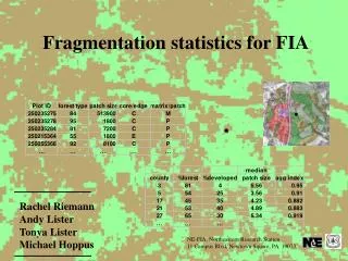
Comparisons… Next, at the scales at which the basics of landuse context appeared to be reasonable (and/or are of interest), comparing a few more variables we’d next most like to have… -- e.g. some of the distribution/configuration variables like patch areas, isolation/aggregation… • Results: • patch sizes differ considerably • NLCD’92 is missing a large percentage of the medium-sized patches – lots of very small ones (1-5 pixels) and one enormous one (e.g. a connected matrix of forest)
Comparisons… Computing with just core forest areas appears to bring the results for patch size statistics much more into line… NLCD’92 NLCD’92
Comparisons… MassGIS NLCD’92 all forest core forest
Comparisons… Looking at some other distribution measures, and how NLCD’92 compares to the ‘truth’… Aggregation index (a measure of isolation) * Avg. corrected perimeter:area ratio (a measure of shape) * *calculated on the core forest area
Comparisons… Looking at the context of developed landuses in an area: as a % of total area as a % of total forest edge
Conclusions/results so far… • Context information in terms of % land cover/land use by area and by edge are both probably useful measures that are reasonably accurate at the county level (as long as being within 2% for ag, 4% for residential, and 6% for forest is okay…). • The classification errors such as residential with trees being classed as forest need to be corrected • For distribution measures -- the per-pixel classification of the NLCD’92 wreaks havoc with the patch size calculations –. • Use of just core forest area in patch size statistics helped considerably. • The task of developing frag statistics for FIA will be iterative –want to run this test again in the Delaware Water Gap area where we have more detailed ground truth (e.g. residential with % tree cover, etc…) • Want to test the NLCD2000 dataset (in the pilot stage) for its frag accuracy • Want to look at this frag information along with other data –e.g. forest types – which are most being affected, incidence of disease… • For metrics that we want but aren’t sufficiently accurate, what other sources are there?
Example management guidelines… http://birds.cornell.edu/conservation/tanager/atlantic.html
Other projects working on frag issues… • (as well as individual researchers…) • E.g… • CSEES – research • NEMO – application • NAUTILUS – research • YFF – application • Cornell Lab of Ornithology – application • BES – • Oakridge ONL – research
Quick check…How related to FIA stats? First quickly checking the datasets against the FIA data in terms of % forest at the county level (1985 and 1998 FIA data) Both the NLCD’92 and MassGIS datasets plotted fairly closely to the FIA statistics at the county level (--within 6%…)