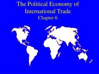
The Political Economy of International Trade Cooperation

1. The Political Economy of International Trade Cooperation READING ASSIGNMENT: Oatley – Chapter 3 Suggested (not required) further reading: Grieco, Joseph M. and John Ikenberry. 2003. The Economics of International Trade. In Grieco and Ikenberry, State Power and World Markets: The International Political Economy. New York: W.W. Norton & Co. pp19-56.

2. Plan • Building blocks (indifference curves, MRS, production frontiers MRT) • Opportunity costs & Comparative advantage • Factor endowments & Hecksher-Ohlin Model • Prisoner’s dilemma

3. Building blocks • Consumption indifference curves • Production possibility frontiers • Analysis of optimized production-consumption equilibrium (without trade)

4. Consumption indifference curves • Consumption  happiness  (UTILITY) • More is better! • But indifferent between some baskets • E.g. U (2 pairs of shoes & 2 Dell desktop computers) = U (6 pairs of shoes & 1 Dell desktop computer) • For our purposes, we’ll consider aggregate "national" consumption indifference curves

6. Points A, B, C, & D provide the country with the same level of “satisfaction.” • Why curved? • Declining marginal utility from consumption • D to C: • If you are at D, you’ll sacrifice 2 million computers for just 10 million shoes • B to A: • If you are at B, you’ll sacrifice 2 million computers only if compensated with 40 million shoes • DECLINING MARGINAL RATE OF SUBSTITUTION • Any point along U1 beats any point along U0 – you want to move to the highest indifference curve

7. Budget Constraint? Slope of this line is the MARGINAL RATE OF PRODUCT TRANSFORMATION

8. Putting the two together

9. Production possibilities frontier • Opportunity costs  negative slope • Straight line  constant opportunity costs • Increasing opportunity costs? • Arise under decreasing returns to scale • Suppose a trade-off between rice and grapes • Some land more suitable for rice than grapes and vice versa • Suppose you start out with all grapes • If you want to switch to rice, you begin with the best land for rice/worse land for grapes • Eventually, you will run out of good-rice-land, and start taking good-grape-land • The opportunity cost of switching to rice increases and increases

11. Movement from P to C (increasing computer production from 0 to 4 million computers) reduces shoe production only by 10 million • But movement from D to Q (again increasing computers by 4 million) reduces shoe production by 100 million! • INCREASING MARGINAL RATE OF PRODUCT TRANSFORMATION

12. Optimizing under autarky (no trade) • Given our preferences (consumption indifference curves) • And our production possibility frontier, • Where to we maximize our utility?

14. Answer MARGINAL RATE OF SUBSTITUTION = MARGINAL RATE OF PRODUCT TRANSFORMATION MRS = MRT

15. Why do countries engage in trade? • Ricardian model: 2 countries, 2 goods & CONSTANT opportunity costs • Logic of COMPARATIVE ADVANTAGE

16. Example is a li’l out of date… • One American worker can produce more computers or more shoes than one Brazilian worker • US has an ABSOLUTE ADVANTAGE in both computers and shoes • So why trade?

17. Differences in opportunity costs! • Suppose we move one American worker from Computers to Shoes • We lose 50 computers for 200 shoes • For each additional pair of shoes produced, the US must forgo 0.25 computers (50/200=¼) • The (constant) opportunity cost of each pair of shoes is ¼ computer • The (constant) opportunity cost of each computer is 4 pairs of shoes (200/50=4)

18. Differences in opportunity costs! • Suppose we move one Brazilian worker from Computers to Shoes • We lose 5 computers for 175 shoes • For each additional pair of shoes produced, Brazil must forgo 0.03 computers (5/175=0.029) • The (constant) opportunity cost of each pair of shoes is 0.03 computer • The (constant) opportunity cost of each computer is 35 pairs of shoes (175/5=35)

19. Critical point • Where is it RELATIVELY cheaper to produce computers? • In the US it costs 4 shoes • In Brazil it costs 35 shoes • Where is it RELATIVELY cheaper to produce shoes? • In the US it costs ¼ computer • In Brazil it costs 0.03 computer

20. Under trade, we may negotiate terms of trade where MRT= –100/10 = –10 or –175/17.5= –10 In autarkic Brazil, the (constant) MRT= –175/5= –35 In autarkic US, the (constant) MRT= –200/50= –4

23. Terms of trade • Obviously the US wants more than 4 pairs of shoes per computer (because this is its autarkic MRT) • Obviously Brazil wants computers for less than 35 pairs of shoes • How do we get to the compromise of 10?

24. Key problems • Why don’t we observe full specialization in one good per country? • Why do some countries have a comparative advantage in some goods and not others?

25. Neoclassical model: 2 countries, 2 goods, increasing opportunity costs

27. US is at EaA (“autarkic America”) • Brazil is at EaB (“autarkic Brazil”) • “Satisfaction” is at U0A & U0B, respectively • With trade, US shifts towards more computer production, Brazil towards shoes • As they shift, however, OPPORTUNITY COSTS INCREASE

30. Where do they stop? • We continue until MRT(A)=MRT(B)=MRS(A)=MRS(B) • Suppose “markets clear” at an exchange ratio of 1 computer for 6 pairs of shoes (light line in the figures) • Countries move to CtA and CtB, respectively, and get U1A and U1B

31. Why don’t we get complete specialization? • Specialization and trade eventually eliminate the differences with regard to opportunity costs between goods (because of increasing opportunity costs)

32. Why does one country have a comparative advantage in one area? Heckscher-Ohlin: Two basic kinds of countries

33. Why does one country have a comparative advantage in one area? • Heckscher-Ohlin: • Compared to the availability of capital & labor in one country, another country will have relatively more or less • Capital-abundant countries: Cost of capital relative to wages is lower • Labor-abundant countries: Wages relative to cost of capital is lower • H-O suggests that countries have an advantage in producing different commodities because of the different factor endowments of countries and the different mixtures of these factors involved in production of different commodities Question regarding “relatively capital abundant” vs “relatively labor abundant” … “relative” to what? • Other countries? Or relative to the other factor? • (Both)

34. Recall a key point • What drives comparative advantage? • It is not differences in the cost of any single factor of production, • but differences in the cross-national relative-abundance • and thus the cross-national relative costs of factors of production • So, even if Americans can make more shoes and more computers (absolute advantages in both), they should still shift to exporting computers and importing shoes

35. So why is there protectionism? • We’ll talk about Stolper-Samuelson and LOSERS from trade next time • For now… prisoner’s dilemma? • Discuss – is unilateral trade opening advantageous?

36. PD settings? • Prisoner's dilemma • http://www.youtube.com/watch?v=ED9gaAb2BEw&feature=related • http://www.youtube.com/watch?v=p3Uos2fzIJ0

37. Prisoner's Dilemma: • A non-cooperative, non-zero-sum game. (Mixed game of cooperation and conflict.) • Individual rationality brings about collective irrationality.

38. Example… • You're reading Tchaikovsky's music on a train back in the USSR. • KGB agents suspect it's secret code. • They arrest you & a "friend" they claim is Tchaikovsky. • "You better tell us everything. We caught Tchaikovsky, and he's already talking…"

39. You know that this is ridiculous – they have no case. • But they may be able to build a case using your testimony and "Tchaikovsky's." • If you "rat" out your "friend" – they will reduce your sentence. • If not, they will throw the book at you.

40. Player 2’s “sucker’s payoff” Player 1’s “sucker’s payoff” Pareto optimal Nash equilibrium (Pareto sub-optimal)

41. Pareto optimality: • No one can be made better off without someone being made worse off • Any change to make any person better off would make someone else worse off • Nash equilibrium: • Every individual pursues his best strategy set, given the strategies of all other players • No one would unilaterally defect • If each player has chosen a strategy and no player can benefit by changing his or her strategy while the other players keep theirs unchanged, then the current set of strategy choices and the corresponding payoffs constitute a Nash equilibrium

42. Individual rationality  collective sub-optimality • The same situation can occur whenever “collective action” is required • The collective action problem is also called the “n-person prisoner's dilemma” • Also called the “free rider problem” • “Tragedy of the commons” • All have similar logics and a similar result: • Individually rational action leads to collectively suboptimal results

43. Is cooperation ever possible in Prisoner's Dilemma? • Yes  • In repeated settings • Axelrod, Robert M. 1984. The Evolution of Cooperation. New York: Basic Books. • Example set of strategies? • Tit-for-tat

44. PD Example from the book • Trade liberalization between US and China

45. China: P,L>L,L>P,P>L,P US: L,P>L,L>P,P>P,L

46. Root of the imbalance between China and USaccording to different theoretical approaches

47. Root of the imbalance between China and USaccording to different theoretical approaches

48. Root of the imbalance between China and USaccording to different theoretical approaches

49. Root of the imbalance between China and USaccording to different theoretical approaches

50. Root of the imbalance between China and USaccording to different theoretical approaches