Download
1 / 58
580 likes | 704 Vues
This study explores the critical challenges inherent in multiscale computation, focusing on various application areas including quantum chromodynamics (QCD), molecular dynamics, and turbulence modeling. It addresses major scaling bottlenecks, such as the interaction among numerous variables and the inefficiencies from local processing. Advanced solutions, including multigrid and algebraic multigrid (AMG) methods, are presented for solving complex partial differential equations (PDEs), along with strategies for optimizing computational performance across different scales.

E N D
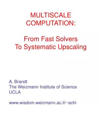
MULTISCALE COMPUTATION:From Fast SolversTo Systematic Upscaling A. Brandt The Weizmann Institute of Science UCLA www.wisdom.weizmann.ac.il/~achi
Major scaling bottlenecks:computing Elementary particles (QCD) Schrödinger equationmoleculescondensed matter Molecular dynamicsprotein folding, fluids, materials Turbulence, weather, combustion,… Inverse problemsda, control, medical imaging Vision, recognition
Scale-born obstacles: • Many variablesn gridpoints / particles / pixels / … • Interacting with each otherO(n2) • Slowness Slowly converging iterations / Slow Monte Carlo / Small time steps / … • due to • Localness of processing
small step Moving one particle at a timefast local ordering slow global move
Solving PDE: Influence of pointwise relaxation on the error Error of initial guess Error after 5 relaxation sweeps Error after 10 relaxations Error after 15 relaxations Fast error smoothingslow solution
Scale-born obstacles: • Many variablesn gridpoints / particles / pixels / … • Interacting with each otherO(n2) • Slowness Slowly converging iterations / Slow Monte Carlo / Small time steps / … • due to • Localness of processing 2. Attraction basins
E(r) r Optimizationmin E(r) multi-scale attraction basins
Scale-born obstacles: • Many variablesn gridpoints / particles / pixels / … • Interacting with each otherO(n2) • Slowness Slowly converging iterations / Slow Monte Carlo / Small time steps / … • due to • Localness of processing 2. Attraction basins Removed by multiscale processing
Solving PDE: Influence of pointwise relaxation on the error Error of initial guess Error after 5 relaxation sweeps Error after 10 relaxations Error after 15 relaxations Fast error smoothingslow solution
h LU = F LhUh = Fh 2h L2hU2h = F2h L2hV2h = R2h 4h L4hV4h = R4h
Multigrid solversCost: 25-100 operations per unknown Linear scalar elliptic equation (~1971)
Multigrid solversCost: 25-100 operations per unknown Linear scalar elliptic equation (~1971) Nonlinear FAS (1975)
h LhUh = Fh LU = F 2h U2h = Uh,approximate +V2h L2hV2h = R2h L2hU2h = F2h Fine-to-coarse defect correction 4h L4hU4h = F4h
Multigrid solversCost: 25-100 operations per unknown Linear scalar elliptic equation (~1971)* Nonlinear Grid adaptation General boundaries, BCs* Discontinuous coefficients Disordered: coefficients, grid (FE) AMG Several coupled PDEs* (1980) Non-elliptic: high-Reynolds flow Highly indefinite: waves Many eigenfunctions (N) Near zero modes Gauge topology: Dirac eq. Inverse problems Optimal design Integral equations Statistical mechanics Massive parallel processing *Rigorous quantitative analysis (1986) (1977,1982) FAS (1975) Withinonesolver
Multigrid solversCost: 25-100 operations per unknown Linear scalar elliptic equation (~1971)* Nonlinear Grid adaptation General boundaries, BCs* Discontinuous coefficients Disordered: coefficients, grid (FE) AMG Several coupled PDEs* (1980) Non-elliptic: high-Reynolds flow Highly indefinite: waves Many eigenfunctions (N) Near zero modes Gauge topology: Dirac eq. Inverse problems Optimal design Integral equations Statistical mechanics Massive parallel processing *Rigorous quantitative analysis (1986) (1977,1982) FAS (1975) Withinonesolver
Same fast solver Local patches of finer grids • Each level correct the equations of the next coarser level • Each patch may use different coordinate system and anisotropic grid “Quasicontiuum” method [B., 1992] and differet physics; e.g.atomistic • Each patch may use different coordinate system and anisotropic grid anddifferent physics; e.g. Atomistic
Multigrid solversCost: 25-100 operations per unknown Linear scalar elliptic equation (~1971)* Nonlinear Grid adaptation General boundaries, BCs* Discontinuous coefficients Disordered: coefficients, grid (FE) AMG Several coupled PDEs* (1980) Non-elliptic: high-Reynolds flow Highly indefinite: waves Many eigenfunctions (N) Near zero modes Gauge topology: Dirac eq. Inverse problems Optimal design Integral equations Statistical mechanics Massive parallel processing *Rigorous quantitative analysis (1986) (1977,1982) FAS (1975) Withinonesolver
Multigrid solversCost: 25-100 operations per unknown Linear scalar elliptic equation (~1971)* Nonlinear Grid adaptation General boundaries, BCs* Discontinuous coefficients Disordered: coefficients, grid (FE) AMG Several coupled PDEs* (1980) Non-elliptic: high-Reynolds flow Highly indefinite: waves Many eigenfunctions (N) Near zero modes Gauge topology: Dirac eq. Inverse problems Optimal design Integral equations Statistical mechanics Massive parallel processing *Rigorous quantitative analysis (1986) (1977,1982) FAS (1975) Withinonesolver
ALGEBRAIC MULTIGRID (AMG) 1982 Coarse variables - a subset 1. “General” linear systems 2. Variety of graph problems
Graph problems Partition: min cut Clustering bioinformatics Image segmentation VLSI placement Routing Linear arrangement: bandwidth, cutwidth Graph drawing low dimension embedding Coarsening: weighted aggregation Recursion: inherited couplings (like AMG) Modified by properties of coarse aggregates General principle: Multilevel objectives
Multigrid solversCost: 25-100 operations per unknown Linear scalar elliptic equation (~1971)* Nonlinear Grid adaptation General boundaries, BCs* Discontinuous coefficients Disordered: coefficients, grid (FE) AMG Several coupled PDEs* (1980) Non-elliptic: high-Reynolds flow Highly indefinite: waves Many eigenfunctions (N) Near zero modes Gauge topology: Dirac eq. Inverse problems Optimal design Integral equations Statistical mechanics Massive parallel processing *Rigorous quantitative analysis (1986) (1977,1982) FAS (1975) Withinonesolver
1D Wave Equation: u”+k2u=f 2p/w wavelength 2h h Non-local components: eiwx,w ≈ ±k Slow to converge in local processing The error afterrelaxation v(x) = A1(x)eikx + A2(x) e-ikx A1(x), A2(x) smooth Ar(x) are represented on coarser grids: A1 + 2 i k A1′ = f1 = rh(x)e-ikx
2D Wave Equation: Du+k2u=f Non-local: w2 (a3,b3) (a2,b2) (a1,b1) (a4,b4) k w1 (a5,b5) (a8,b8) (a7,b7) O(H) (a6,b6) ei(w1x + w2y) w12+ w22≈ k2 On coarser grid (meshsize H): • Fully efficient multigrid solver • Tends to Geometrical Optics • Radiation Boundary Conditions: directly on coarsest level
Generally: LU=F Non-local part of U has the form m Σ Ar(x) φr(x) r = 1 L φr ≈ 0 Ar(x) smooth {φr } found by local processing Ar represented on a coarser grid
Multigrid solversCost: 25-100 operations per unknown Linear scalar elliptic equation (~1971)* Nonlinear Grid adaptation General boundaries, BCs* Discontinuous coefficients Disordered: coefficients, grid (FE) AMG Several coupled PDEs* (1980) Non-elliptic: high-Reynolds flow Highly indefinite: waves Many eigenfunctions (N) Near zero modes Gauge topology: Dirac eq. Inverse problems Optimal design Integral equations Statistical mechanics Massive parallel processing *Rigorous quantitative analysis (1986) (1977,1982) FAS (1975) Withinonesolver
N eigenfunctions Electronic structures (Kohn-Sham eq): i = 1, …, N= # electrons O(N) gridpoints per yi O(N2 ) storage Orthogonalization O(N3) operations Multiscale eigenbase 1D: Livne O(NlogN) storage & operations V = Vnuclear+ V(y) One shot solver
Multigrid solversCost: 25-100 operations per unknown Linear scalar elliptic equation (~1971)* Nonlinear Grid adaptation General boundaries, BCs* Discontinuous coefficients Disordered: coefficients, grid (FE) AMG Several coupled PDEs* (1980) Non-elliptic: high-Reynolds flow Highly indefinite: waves Many eigenfunctions (N) Near zero modes Gauge topology: Dirac eq. Inverse problems Optimal design Integral equationsFull matrix Statistical mechanics Massive parallel processing *Rigorous quantitative analysis (1986) (1977,1982) FAS (1975) Withinonesolver
Integro-differential Equation differential , dense Multigrid solver Distributive relaxation: 1st order 2nd order Solution cost ≈ one fast transform(one fast evaluation of the discretized integral transform)
Integral Transforms G(x,x) Transform Complexity O(n logn) Fourier Laplace O(n logn) O(n) Gauss Potential O(n) G(x,x) * Exp(ikx) O(n logn) Waves
G(x,y) Glocal Gsmooth s |x-y| ~ 1 / | x – y | G(x,y) = Gsmooth(x,y) + Glocal(x,y) s ~ next coarser scale O(n) not static!
Multigrid solversCost: 25-100 operations per unknown Linear scalar elliptic equation (~1971)* Nonlinear Grid adaptation General boundaries, BCs* Discontinuous coefficients Disordered: coefficients, grid (FE) AMG Several coupled PDEs* (1980) Non-elliptic: high-Reynolds flow Highly indefinite: waves Many eigenfunctions (N) Near zero modes Gauge topology: Dirac eq. Inverse problems Optimal design Integral equations Statistical mechanics Monte-Carlo Massive parallel processing *Rigorous quantitative analysis (1986) (1977,1982) FAS (1975) Withinonesolver
Multiscale ~ DiscretizationLattice for accuracy Monte Carlocost ~ “volume factor” “critical slowing down” Multigrid moves Many sampling cycles at coarse levels
Multigrid solversCost: 25-100 operations per unknown Linear scalar elliptic equation (~1971)* Nonlinear Grid adaptation General boundaries, BCs* Discontinuous coefficients Disordered: coefficients, grid (FE) AMG Several coupled PDEs* (1980) Non-elliptic: high-Reynolds flow Highly indefinite: waves Many eigenfunctions (N) Near zero modes Gauge topology: Dirac eq. Inverse problems Optimal design Integral equations Statistical mechanics Massive parallel processing *Rigorous quantitative analysis (1986) (1977,1982) FAS (1975) Withinonesolver
Same fast solver Local patches of finer grids • Each level correct the equations of the next coarser level • Each patch may use different coordinate system and anisotropic grid “Quasicontiuum” method [B., 1992] and differet physics; e.g.atomistic • Each patch may use different coordinate system and anisotropic grid anddifferent physics; e.g. Atomistic
Repetitive systemse.g., same equations everywhere UPSCALING: Derivation of coarse equationsin small windows
Scale-born obstacles: • Many variablesn gridpoints / particles / pixels / … • Interacting with each otherO(n2) • Slowness Slowly converging iterations / Slow Monte Carlo / Small time steps / … • due to • Localness of processing • Attraction basins Removed by multiscale processing
Systematic Upscaling • Choosing coarse variables • Constructing coarse-leveloperational rules equations Hamiltonian
Macromolecule ~ 10-15 second steps
Systematic Upscaling • Choosing coarse variablesCriterion: Fast convergence of “compatible relaxation”
Systematic Upscaling • Choosing coarse variablesCriterion: Fast equilibration of “compatible Monte Carlo” OR: Fast convergence of “compatible relaxation” Local dependence on coarse variables • Constructing coarse-leveloperational rules Done locally In representative “windows” fast
Macromolecule Two orders of magnitude faster simulation
Total mass • Total momentum • Total dipole moment • average location Fluids