Download
1 / 42
430 likes | 591 Vues
Superconducting gravimetry at Onsala Space Observatory. The first year June 13, 2009 – Status August 31, 2010. Basic facts. Big- G : Mass attracts mass with a force –( G m 1 m 2 )/ r 2 (G is Newton’s constant of gravity , G = 6.67 ·10 -11 m 3 /kg s 2

E N D
Superconducting gravimetryat Onsala Space Observatory The first year June 13, 2009 – Status August 31, 2010
Basic facts • Big-G: Massattractsmass with a force –(G m1m2)/r2 (G is Newton’sconstant of gravity, G = 6.67 ·10-11 m3/kg s2 • If you are familiar with vectors, = – (G m1m2)/r3 • Little-g: A massive sphere (~earth) generates an accelaration of an object at the surface of -g = –(G mE)/R2 = - 9.81… m/s2 (minus for downward)mEsphere’smass, Ritsradius • On Earth, rotating and slightlyflattened, centrifugal acceleration combines with the attraction, lowering it by roughly 0.34% whengoing from pole to equator. At Onsala, g = 9.817 159 m/s2 • Vertical gradient of gravity:If you climb up, little-gdecreases with dg/dr = -2 g/R or -3.08 µm/s2 per meter • The Gal unit(after Galileo), an antiquity from the CGS era: g = 981… Gal 1 µGal = 10 nm/s2 - Yes, wemeasuredown to 1 nm/s2, and even less.
Gravimeters • Absolute measurements: by time • Revertingpendulum • Ballistic or falling test mass • Relative measurements: measurechange of gravity over time using a restoring force • Metal or quartz spring on a balancebeam and test mass, measure elongation (control by feed-back) • Inducedmagneticfield in a superconducting test mass, measure position (control by feed-back) • Measurement of gravity is along the vertical (actually a tautology); however, the platformmighttilt. A combination of tiltmeters and gravimeter forms a fully 3-dimensional measurement.
One year of gravityrecording: The basic sampling interval is 1s; however, the recordsshownhere are downsamled to 10min. The red curve shows the full signal except that a drift model has beensubtracted. The bluecurveresults after subtraction of a model for tides and polar motion, and the purplecurve after additional removal of air pressure effects. The black curve is identical to the purpleoneexcept that it is drawn at 10 timeslargerscale. The remaining variations seen in the black curve are due to modelinsufficiencies: higher order atmosphericdensitystructure, Kattegat loadingout of hydrostaticbalance, ground water and massflows in the vegetation near the observatory.
One year of gravityrecording: The basic sampling interval is 1s; however, the recordsshownhere are downsamled to 10min. The red curve shows the full signal except that a drift model has beensubtracted. The bluecurveresults after subtraction of a model for tides and polar motion, and the purplecurve after additional removal of air pressure effects. The black curve is identical to the purpleoneexcept that it is drawn at 10 timeslargerscale. The remaining variations seen in the black curve are due to modelinsufficiencies: higher order atmosphericdensitystructure, Kattegat loadingout of hydrostaticbalance, ground water and massflows in the vegetation near the observatory.
Earth tidesocean tidespolar motion Astronomical cause: moon and sun (+planets) Earth elasticresponse (deformation, internalmassredistribution)adds 16%. The tidalgravityfactorδ=1.16.. Moon: 258 nm/s2 Sun: 120 nm/s2 at Onsala Two periods per day (semidiurnal lunar / solar)
Earth tidesocean tidespolar motion • The Nearly-diurnal Free Wobble. The fluid core of the earthperforms a freenutationaround the earths rotation axis. The corerotatessuch that it makes one extra turn in 434 siderealdays. The resonancefrequency of the nearly-diurnalfreewobble, as the phenomenon is called, is thus (1/Ts) × (1+1/434) • This motion implies pressure forces on the core-mantleboundary and internalmassredistribution. It affects the tidalgravityfactor, lowering it from 1.16 to e.g. 1.14 at the K1 tide. And amplifying it at frequencieshigherthan the resonancefrequency. The effect is narrow-banded and affectsonlydiurnaltides.
Earth tidesocean tidespolar motion Ifmoon and sunappearedonly in the equatorial plane, wewould not havebutsemidiurnaltides, M2 (lunar) and S2 (solar). The inclinations of the ecliptic and the lunar orbit cause the appearance of the bodies at different declinationsabove and below the equatorial plane during (solar, lunar) day and night, respectively. This gives rise to the diurnaltides, i.e. one period per (lunar, solar) day. The tidenamed K1 is such an example (period = 1 siderealday). The tidal oscillation patterns in the oceans dependstrongly on the periods of excitation.
Earth tidesocean tidespolar motion Ocean tideloadingeffects: The movingmass in the ocean tideacts on a gravimeter at distance by Massattraction Deformation of the earthcrust and ensuingchange of gravity as instrument is movedthrough the verticalgravity gradient. Solid earthmassredistribution, which provides a secondaryattractioneffect. At Onsala, the global ocean tide M2 causes a gravity variation of 6.24 nm/s2 (K1: 2.58 nm/s2). These are valuesderived from the modelshown to the left (FES2004, T. Letellier). The dominatinginfluence is from the seanear-by.
Earth tidesocean tidespolar motion The orbits of the bodies, in particular the moon’s, are still morecomplicated. In addition to inclination, the lunar orbit is elliptical, its ellipticity changes, and the inclinationchangestoo as the sunexcerts a variable pull. And the nodeline, whereorbit and eclipticintersect, is slowly turning, onecycle in 14.6 years in a retrograde sense. Orbitinclinationalsoimplies that the bodiesexcert different tidal pull on the earthwhenthey are once in the high part of the orbit and another time in an equatorial transit. Thus, there are alsotideeffects at basicallytwocycles per month (lunar, Mf) and per year (solar, Ssa). All in all there is an infinite number of harmonics(sines and cosines) needed to completelyrepresent the tidaleffects over time. The diagrams show the logarithm of the amplitude of the tide potential constituents. The amplitudes are given in meters (elevation of an equlibrium ocean) .
Earth tides ocean tidespolar motion Chandler Wobble, AnnualWobble. The instataneous rotation axis of the earthperforms an errantpatharound the axis of figure (the meanpole position), completing a turn in 435 days (seefigure to the left). This is a freeresonanceof a rotating, flattenedbody. It can be observed in a toy gyro when you gently and shortlytapagainst the axis. The wobbledecaysquickly. In the earth it is primarily the changingweather (winds and pressure areas) that are able to excite and steadilynurish the wobble. At onecycle per year, weatherpatternshave a stronng repetition (e.g. the high-low pressure changeoccuring in Sibereabetweenwinter and summer). The annualweatherpatternsgenerate a forcedwobble at 365.25 days period. The combinedfree and forced motion of the axis is called Polar motion.
Earth tides ocean tidespolar motion Polar motion implies a change in little-gsince the shortestdistance of an observer from the axis of rotation is changing. As this distancechanges so does centrifugal acceleration. The effectcan not be felt at the pole and at the equator. You can look upon polar motion as a change of (the true) geographiclatitude. Say the pole offset is 3m. The maximum effect at midlatitude is then (2π/Ts)2Δr = 16 nm/s2whereT = length of siderealday. Although it takes 14 months for onecycle, the effect is measurable as wewillsee.
Atmosphericeffectsmassattraction and loading • Like under the load of the ocean tide, the earth dips also under the variable load of air pressure. However, the mass of the load is distributed in a verticalcolumn, and if it is close to a gravimeter, the masses at height are moreefficientthanthosenear the ground to pull at the gravimeter.
Hydrodynamic Loading • Where air pressure acts on the ocean surface, the water adjusts so that the pressure at the ocean bottom remainsconstant. This is the so-calledinverse barometer effect. So, air pressure above ocean would not deform the earth, although the sealevelwouldchange. • However the ocean needs time to adjust. The shallower the water and the narrower the straights, the longer is the time for adjustment. • Windfields and fast travellinglow-pressure systems excite oscillations in basins and pile up water at the coast. • Thus, near the shores of shallow, semi-enclosedbasins the sealevel is in hydrostaticbalanceonly on the time scale of days to weeks. The misadjustmentcausesloading and massattraction.
Ground water and biosphere • Variable ground water masses and the water cycle in the biospherecanimplymasschanges in the verynearenvironment of a gravimeter station. Especiallyground water presents a serious problem ifhydrology is considered a source of noise (while the measurement of ground water variations with a gravimeter is a clumsy and expensivemethod) . • The gravimeter lab at Onsala is situated on crystallinebedrock, which is expected to host small water masses. Precautionsduringconstructionprevent the accumulation of rain water. It is collected in an underground pond and pumpedaway by controlling a constant water level in the pond. • However, the forest (trees, undervegetation, soil) on the neighbourground is out of the observatory’scontrol. Here, wewillhave to deal with seasonal perturbations duemostly to the vegetation.
InstrumentGWR (Goodkind & Warburton, San Diego, Cal.) • Principle • Features • Sensor Drift • Signal-to-noise
Invarroddown to 4 m depthrecordsverticalsurface motion (thermal expansion, annual period) Coredborehole ~20m depth, typical water surface at 2m below rock surface; water level (pressure) sensor (installation in process) Temperaturesensors are installed in SCG platform and in the rock basement at 4 m depth. The room air conditioner and fan system circulates air also to the basement rock surface
Puddlebeforebeingdrained by channeling, locationcoincident with northernwall of the building. The coredborehole (red metal cover) is visible in the foreground.
Investigation of bedrockfractures The site is on a bedrockoutcrop, low-grademetamorphicgneis Initial GPR investigation to locatefractures, found a conspicuoussubhorizontalstructure at 2.0 – 2.3 m depth; in all three major fracturegroups with strike/dip as follows • group 1: 80º/70º • group 2: 285º/85º • group 3: 300º/20º Fracturefrequencyindicator (RQD) = 90 (90-100 verygood, 10-25 poor) . GeotechnicalQ-value: 10 – 40 typical, 2 to 6 in the fracturezones.
Water drainage • Drainage experiment in the coredborhole: Intervals of 3 m • ”The rock is tight” Exception in depth segment 3.5 – 6.5 m wheredrainage hints at openfractures at 6 m depth • Groundwaterlevel at 1 - 1.5 m belowsurface, followstopography • Expect water pressure from highertopography east of building to stabilize water level in bedrockbody
Cryogenic sensor • Feedback loop • Feedback controlledlevelling • 60 l liquid helium dewar • Coldheadgeneratesliquid from room-temperatureHe gas.
Relative measurement Sensor factor is not related to principal SI units. The instrument needscalibration (next page). There is also a slowlyincreasingeffect in sensitivity, showing as a virtualdecrease of gravity, first exponentiallydecaying, assymptotically as a linearfunction of time. This is calleddrift.
The drift model A + B t + Cexp(-D t) B = 0.014 6 nm/s2/h C = 182 nm/s2 1/D = 474 h (typicalresults)
Verticality Note the tiltactuators marked VX and VY on the photo to the left. The diagrams below show the action of the tilt controllers duringthe Rayleighwave motion from the Mauleearthquake (Chile, Feb. 27, 2010).
This is about the smallestmagnitudeearthquake that engauges the SCG’s tiltcontrol. The epicentre of this event is not far from ourantipode. Source time was 17:56:19
Seismology: Free Oscillations The gravimeter data acquisitionunit has a special filter channel that band-passesthosestandingwaves, a.k.a. Free Oscillations orSeismic Normal Modes, that are excited in major earthquakes (example is from Andaman event Aug. 10, 2009). The Free Oscillation spectrum covers periods from 1.5 to 54 minutes.
After the Magnitude 8.8 - Earthquake offshore Maule, Chile, 2010-Feb-27 at 06:34:14 UTC Comparison of Free Oscillation spectrum at Onsala with theoretical models. “S” stands for Spheroidal mode, right-subscript spherical harmonic degree, and left-subscript overtone number (number of nodes on earth radius. Splitting of modes relates to Coriolis effect. 0S2 is notoriously hard to observe.
East North Vertical Guralp 120s at Onsala
GIA – glacial isostaticadjustment • Research target for an AG project • AG calibrates SCG Isostasy = a solid bodywithoutinternalforces that changeitsshape and gravityfield. GIA is the visco-elasticrebound after glacial loadingand unloading. The earthreturnsslowly to itspre-loadingshape. Gravityanomaly (internalbuoyancy) provides the force, visco-elasticity the resistance. The oceans with their variable massadjust to the ambient gravityfield and at the same time provides a dynamicload. Peripheral to the upliftingdome is a subsidingtrough, an effect of the elasticity of the lithosphere (top ~200 km of the earth). Ratio of central upliftversusperipheralsubsidence ~10 : 1 (mm/yr) in and around Fennoscandia.
Land uplift implies a gravity change:between -1.7 and -2 nm/s2 per mm NKG Nordic Geodetic Commission Absolute-gravity plan (2000--) Participants from SE, NO, FI, DK, DE Calibration sites: Preferably Fundamental- geodetic sites (Metsähovi, NyÅlesund, Onsala) • Intercomparison of Absolute gravimeters • Monitor temporal variations Gitlein, 2009, IfE Hannover
Δg ~ -1.7 nm/s2 per mmland uplift -3 nm/s2 is due to pure uplift. ~1.3 nm/s2 is due to earth mantle density in the competent layer (where is it?) And on the extent of the ice sheet BIFROST project: Crustal motion verticalcomponentdetermined from GPS (Lidberg et al., 2010) interpolatedusing a thick-plate approach that minimizes deformation and buoyancyenergy
The SCG residuals in threeflavoursusing different models for the instrumental drift and an empirical or a nominal model, respectively, for long-period solar tides. Four episodes of AG measurements (minus 981715900 nm/s2) are shown with yellow-and-redcircles and greyerror bars. ”GIA” is gravity rate of changebased on BIFROST GPS (Lidberg et al., 2010) 4.05 ± 0.44 mm/yr and converted to gravityusing a ratio of -2 nm/s2/mm
SCG Calibration The tidal variations, prefarablyduringnew-moon in summer or full-moon in winter, are used to determine a scalefactor for the SCG readings. In the diagram above the Absolute Gravimeter readings (red dots) havebeenseparatedvertically for legibility. SCG readings are shown in light green (1s- samples) and by greycircles (low-passed and resampled at 900s).
Fundamental Geodetic Station • GGOS – Global GeodeticObserving Systems • Coordination: VLBI, GNSS, Gravimeter , Tide gauge (+SLR +DORIS +) • Latest addition: Guralp 120s 3-comp. Seismometer (SNSN – Swedish National Seismic Network, Uppsala university) The threepillars of geodesy: