Information complexity and exact communication bounds
480 likes | 710 Vues
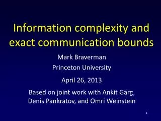
Information complexity and exact communication bounds. Mark Braverman Princeton University. April 26, 2013. Based on joint work with Ankit Garg , Denis Pankratov , and Omri Weinstein. Overview: information complexity. Information complexity :: communication complexity a s

Information complexity and exact communication bounds
E N D
Presentation Transcript
Information complexity and exact communication bounds Mark Braverman Princeton University April 26, 2013 Based on joint work with Ankit Garg, Denis Pankratov, and Omri Weinstein
Overview: information complexity • Information complexity :: communication complexity as • Shannon’s entropy :: transmission cost
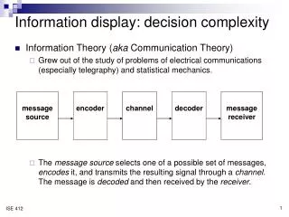
Background – information theory • Shannon (1948) introduced information theory as a tool for studying the communication cost of transmission tasks. communication channel Bob Alice
Shannon’s entropy • Assume a lossless binary channel. • A message is distributed according to some prior . • The inherent amount of bits it takes to transmit is given by its entropy . X communication channel
Shannon’s noiseless coding • The cost of communicating many copies of scales as . • Shannon’s source coding theorem: • Let be the cost of transmitting independent copies of . Then the amortized transmission cost .
Shannon’s entropy – cont’d • Therefore, understanding the cost of transmitting a sequence of ’s is equivalent to understanding Shannon’s entropy of . • What about more complicated scenarios? X communication channel Y • Amortized transmission cost = conditional entropy .
Easy and complete! A simple example • Alice has uniform • Cost of transmitting to Bob is • Suppose for each Bob is given a unifomly random such that then… cost of transmitting the ’s to Bob is .
Meanwhile, in a galaxy far far away… Communication complexity [Yao] • Focus on the two party randomized setting. Shared randomness R Y X A & B implement a functionality . A F(X,Y) B e.g.
Communication complexity Goal: implement a functionality . A protocol computing : Shared randomness R Y X m1(X,R) m2(Y,m1,R) m3(X,m1,m2,R) A B F(X,Y) Communication cost = #of bits exchanged.
Communication complexity • Numerous applications/potential applications (streaming, data structures, circuits lower bounds…) • Considerably more difficult to obtain lower boundsthan transmission (still much easier than other models of computation). • Many lower-bound techniques exists. • Exact bounds??
Communication complexity • (Distributional) communication complexity with input distribution and error : Error w.r.t. . • (Randomized/worst-case) communication complexity: . Error on all inputs. • Yao’s minimax: .
Set disjointness and intersection Alice and Bob each given a set , (can be viewed as vectors in • Intersection . • Disjointness if , and otherwise. • is just 1-bit-ANDs in parallel. • is an OR of 1-bit-ANDs. • Need to understand amortized communication complexity (of 1-bit-AND).
Information complexity • The smallest amount of information Alice and Bob need to exchange to solve . • How is information measured? • Communication cost of a protocol? • Number of bits exchanged. • Information cost of a protocol? • Amount of information revealed.
Basic definition 1: The information cost of a protocol • Prior distribution: . Y X Protocol transcript Protocol π A B what Alice learns about Y + what Bob learns about X
Mutual information • The mutual information of two random variables is the amount of information knowing one reveals about the other: • If are independent, . • . H(B) H(A) I(A,B)
Basic definition 1: The information cost of a protocol • Prior distribution: . Y X Protocol transcript Protocol π A B what Alice learns about Y + what Bob learns about X
Example • is. • is a distribution where w.p. and w.p. are random. Y X MD5(X) [128 bits] X=Y? [1 bit] A B 1 + 64.5 = 65.5 bits what Alice learns about Y + what Bob learns about X
Information complexity • Communication complexity: . • Analogously: .
Prior-free information complexity • Using minimax can get rid of the prior. • For communication, we had: . • For information .
Connection to privacy • There is a strong connection between information complexity and (information-theoretic) privacy. • Alice and Bob want to perform computation without revealing unnecessary information to each other (or to an eavesdropper). • Negative results through arguments.
Information equals amortized communication • Recall [Shannon]: . • [BR’11]: , for . • For : . • [an interesting open question.]
Without priors • [BR’11] For : . • [B’12] .
Intersection • Therefore • Need to find the information complexity of the two-bit !
The two-bit AND • [BGPW’12] bits. • Find the value of for all priors . • Find the information-theoretically optimal protocol for computing the of two bits.
“Raise your hand when your number is reached” The optimal protocol for AND 1 Y{0,1} X{0,1} A If X=1, A=1 If X=0, A=U[0,1] If Y=1, B=1 If Y=0, B=U[0,1] B 0
“Raise your hand when your number is reached” The optimal protocol for AND 1 Y{0,1} X{0,1} A If X=1, A=1 If X=0, A=U[0,1] If Y=1, B=1 If Y=0, B=U[0,1] B 0
Analysis • An additional small step if the prior is not symmetric (). • The protocol is clearly always correct. • How do we prove the optimality of a protocol? • Consider the function as a function of .
The analytical view • A message is just a mapping from the current prior to a distribution of posteriors (new priors). Ex: “0”: 0.6 “1”: 0.4 Alice sends her bit
The analytical view “0”: 0.55 “1”: 0.45 Alice sends her bit w.p½ and unif. random bit w.p½.
Analytical view – cont’d • Denote . • Each potential (one bit) message by either party imposes a constraint of the form: • In fact, is the point-wise largest function satisfying all such constraints (cf. construction of harmonic functions).
IC of AND • We show that for described above, satisfies all the constraints, and therefore represents the information complexity of at all priors. • Theorem: represents the information-theoretically optimal protocol* for computing the of two bits.
*Not a real protocol • The “protocol” is not a real protocol (this is why IC has an infin its definition). • The protocol above can be made into a real protocol by discretizing the counter (e.g. into equal intervals). • We show that the -round IC:
Previous numerical evidence • [Ma,Ishwar’09] – numerical calculation results.
Applications: communication complexity of intersection • Corollary: • Moreover:
Applications 2: set disjointness • Recall: . • Extremely well-studied. [Kalyanasundaram and Schnitger’87, Razborov’92, Bar-Yossef et al.’02]: . • What does a hard distribution for look like?
A hard distribution? Very easy!
A hard distribution At most one (1,1) location!
Communication complexity of Disjointness • Continuing the line of reasoning of Bar-Yossef et. al. • We now know exactly the communication complexity of Disjunder any of the “hard” prior distributions. By maximizing, we get: • , where • With a bit of work this bound is tight.
Small-set Disjointness • A variant of set disjointness where we are given of size . • A lower bound of is obvious (modulo ). • A very elegant matching upper bound was known [Hastad-Wigderson’07]: .
Using information complexity • This setting corresponds to the prior distribution • Gives information complexity • Communication complexity
Overview: information complexity • Information complexity :: communication complexity as • Shannon’s entropy :: transmission cost Today: focused on exact bounds using IC.
Selected open problems 1 • The interactive compression problem. • For Shannon’s entropy we have • E.g. by Huffman’s coding we also know that • In the interactive setting • But is it true that ??
Interactive compression? • is equivalent to , the “direct sum” problem for communication complexity. • Currently best general compression scheme [BBCR’10]: protocol of information cost and communication cost compressed to bits of communication.
Interactive compression? • is equivalent to , the “direct sum” problem for communication complexity. • A counterexample would need to separate IC from CC, which would require new lower bound techniques [Kerenidis, Laplante, Lerays, Roland, Xiao’12].
Selected open problems 2 • Given a truth table for , a prior , and an , can we compute ? • An uncountable number of constraints, need to understand structure better. • Specific ’s with inputs in . • Going beyond two players.
External information cost Y X Protocol transcript Protocol π A C B what Charlie learns about
External information complexity • . • Conjecture: Zero-error communication scales like external information: • Example: for this value is