Scaling Ionograms
950 likes | 1.27k Vues
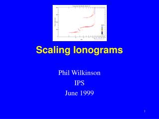
Scaling Ionograms. Phil Wilkinson IPS June 1999. Basic Scaling. Regions of the Ionosphere Normal regions: E, F2, F2 & sporadic E Less familiar: E2, F0.5, F1.5, meteors Notable conditions: spread F, absorption Notorious effects: interference, equipment failure. Basic Scaling.

Scaling Ionograms
E N D
Presentation Transcript
Scaling Ionograms Phil Wilkinson IPS June 1999
Basic Scaling • Regions of the Ionosphere • Normal regions: E, F2, F2 & sporadic E • Less familiar: E2, F0.5, F1.5, meteors • Notable conditions: spread F, absorption • Notorious effects: interference, equipment failure
Basic Scaling • Geometry of reflections • think specular • know the difference between thick and thin layers; retardation and blanketing, • recognise examples of layers • develop concepts of oblique returns; recognise and eliminate them when scaling • recognise unusual things; particle E, spurs, travelling disturbances
Basic Scaling • Resources • UAG-23A; the bible, by Rawer and Piggott • UAG-50; the High Latitude Supplement by Piggott • INAG; an outlet for frustration for some, a link with all the other scalers for others • Japanese scaling manual • Scaling aids • IPS scaling notes • ionograms and your own common sense • look at, and scale, lots of ionograms
Nuts and Bolts of Scaling • Accuracy of the scaling - qualifying letters • quantitative accuracy; E, D, U • unquantifiable errors; J, A, O, Z • unknown errors; I • Reason for the loss of accuracy - descriptive letters • Gaps; A, B, C, G, L, R, S, W, Y • bumps; H, V • things; F, K, P, Q, X, Z • Flags • which are more objective things.
Ionospheric Features • Once you recognise these you are understanding much of the ionogram. • Spread F: a well known night time phenomenon. • sporadic E • Travelling ionospheric disturbances (TID); medium scale features. • Ionospheric storms - These are global events. • Troughs: a sub auroral, large scale features.
Ionospheric Regions • There are distinctive aspects to the different regions • Mid latitudes • sporadic E, travelling ionospheric disturbances, ionospheric storms • Low latitudes • absorption, thick ionosphere and variability, nighttime HF interference • High latitudes • particle effects (Es-K, B) and troughs and ridges of ionisation, much spreading in E and F region
Course Objectives • recognise and scale all the conventional parameters, • use scaling letters effectively, • recognise good and bad ionograms, • use simple principles to scale complex ionograms. • appreciate the sources affecting ionograms, In addition you may • recognise large scale ionospheric processes, • become more confident in assessing ionospheric effects on HF systems.
Sample Ionograms : nighttime • Boring nighttime ionogram • Clear foF2 and fxF2 • Multiples present • No interference effects • A few odd details worth noting: • around the time base echo • slight spreading foF2, fmin, h’F, all Es are easy; fxI is too.
Sample Ionograms : daytime • Typical daytime ionogram • E/F region layers • multiples • extraordinary weak • sporadic E present • easy to scale Scaling problems: • foE - extrapolation • Es - weak traces • fxI - interference
Sample Ionograms : nighttime (Chch 31/05/99 12 UT) • What can we say? • Clear fmin ( __ES) • no Es parameters • Clear foF2, • fxI = foF2+split • h’F, extrapolate down, maybe ( __US) This is the hardest decision you will make scaling ionograms like this.
Sample Ionograms : nighttime (Chch 31/05/99 17 UT) • What can we say? • Clear fmin ( __ES) • no Es parameters • foF2 • Clearly spread F is present, scale inside edge ( __ . F) • fxI - scale outside edge of trace (could be slightly high here) • h’F, extrapolate down, probably ( __. .) • Note: • multiple is spread less • primary appears to be split. • Clear gaps in trace due to interference You ought to be able to scale these better than autoscale did!
Sample Ionograms : nighttime (Hobart 31/05/99 11 UT) • What can we say? • Clear fmin ( __ES) (You can get to like fmin) • no Es parameters (Phew) • foF2 • Clearly spread F is present, scale inside edge ( __ . F) • but did you recognise the Z-trace? • fxI - scale outside edge of the spread F. • h’F, extrapolate down, maybe ( __US) • Note: • multiple is spread less • You can get a good foF2 value from the Z-trace You ought to be able to scale these better than autoscale did!
Sample Ionograms : nighttime (Townsville 31/05/99 16 UT) • What can we say? • Clear fmin ( __ES) • no Es parameters • foF2 • Clearly spread F is present, scale inside edge ( __ UF) • fxI - scale outside edge • h’F, extrapolate down, maybe ( __US) • Note: • More spread • but multiple gives some guidance • multiple has odd shape
Sample Ionograms : nighttime (Townsville 31/05/99 17 UT) • What can we say? • Clear fmin ( __ES) • no Es parameters • foF2 • Clearly spread F is present, scale inside edge ( __ UF) or worse • fxI - scale outside edge • h’F, extrapolate down, maybe ( __ . Q) (for range spread) • Note: • multiple is not much help • traces are now rather broad • interference evident
Sample Ionograms : nighttime (Christchurch 30/05/99 19 UT) • Well developed mid latitude spread F • What is fxI • possibly interference obscures part of the trace, ( __ US ) • Note X-multiple • F/S = 3P
Sample Ionograms : nighttime (Townsville 30/05/99 14 UT) • What can we say? • Clear fmin ( __ES) • no Es parameters • foF2 • Looks awful? Look at multiple, back to primary, and foF2 is clear, and probably not spread. • fxI - scale outside edge. Probably (__ U S). • h’F, extrapolate down, probably ( __ . Q) (for range spread) • Note: • (the black dash/dots were my attempt to identify the main trace) • multiple, once identified, is valuable • many traces are now present, confusing the ionogram • interference very evident (it can get worse)
Sample Ionograms : daytime (Christchurch 31/05/99 03 UT) • What can we say? • Clear fmin ( __ ) (with no scaling letters) (bit high here) • Sporadic E is present • foEs: descending layer, multiple present, extra-ordinary present • fbEs: tip of F region present • foF2: good value • h’F okay • Note: • This is a good daytime ionogram to scale • disturbed multiple • how many sporadic E layers are present?
Sample Ionograms : daytime (Townsville 31/05/99 00 UT) • What can we say? • Clear fmin ( __ ) (with no scaling letters) • Sporadic E parameters are awkward • probably some X component present • a weak trace, and may depend on sequence • foF2: good value • h’F2 okay, h’F possibly disturbed • foE: scaled too low here. • Note: • sporadic E gives problems • This is a typical daytime ionogram, just a little awkward
Sample Ionograms : daytime (Hobart 23/05/99 23 UT) • Clear descending Es layer (but check sequence anyway) • Another Es layers is also present • This is a useful example of several multiples. • Decide which are multiples of which • scale the primary characteristics • Note the possibly second Es layer • ordinary component is hard to detect • but extra ordinary is clear
Sample Ionograms : daytime (Townsville 29/05/99 05 UT) • Fmin? Weak trace rule • foF2: easy, autoscale agrees • h’F2: poorly formed F1, none there • h’F: (__ U A) or (__ UH) or (__ ) ?? • foEs ? How many Es traces and which • foE?
Sample Ionograms : daytime (Townsville 29/05/99 05 UT) • Fmin Weak trace rule - ignore the low bit • but some discussion over this. See a sequence. • foF2: agreed • h’F / h’F2: • h’F: (__ H) only h’F scaled • foEs: scale the highest foEs. Note low type • foE: using c, h Es layers, foe = good value
Sample Ionograms : daytime (Mundaring 02/06/99 02 UT) • Spread Es example • Spreading in the E region is an unusual condition we note by scaling a Q on h’Es • There may also be a slant Es here • Note weak F2 region criticals • Also note the odd splitting on the Mundaring trace. • An example of an equipment problem you would need to recognise.
Sample Ionograms : daytime (Christchurch 24/05/99 23 UT) • Travelling Ionospheric Disturbances (TIDs) • give some zest to scaling. • They affect both the E and F region, • but are most prominent in F2 region. • When present, scale H on characteristics affected by it. • However, this ionogram has several other tricky bits • fmin - weak trace rule needed? • foE - extrapolation, probably ( __ UA) • (and maybe scaled even higher than here) • h’Es - extrapolation ( __ UG)