Download
1 / 47
470 likes | 614 Vues
How to detect the virtually undetectable in the atmosphere. Prof. Dudley Shallcross School of Chemistry. 3 most abundant gases in each planetary atmosphere Jupiter H 2 (93%) He (7%) CH 4 (0.3 %) Saturn H 2 (96%) He (3%) CH 4 (0.45 %) Uranus H 2 (82%) He (15%) CH 4 (2.3 %)

E N D
How to detect the virtually undetectable in the atmosphere. Prof. Dudley Shallcross School of Chemistry
3 most abundant gases in each planetary atmosphere Jupiter H2 (93%) He (7%) CH4 (0.3 %) Saturn H2 (96%) He (3%) CH4 (0.45 %) Uranus H2 (82%) He (15%) CH4 (2.3 %) Neptune H2 (80%) He (19%) CH4 (1-2 %) VenusCO2 (96%) N2 (3.5%) SO2 (0.015 %) Mars CO2 (95%) N2 (2.7%) Ar (1.6 %) Earth N2 (78%) O2 (21%) Ar (0.93 %)
0.9% of mass 9% of mass 90% of mass
UV-A O O O O O O O O O O UV-B
The Chapman Mechanism In the 1930s Sidney Chapman devised a mechanism that accounted for the ozone layer and the temperature structure. O2 + h O + O O + O2 + M O3 + M O3 + hO2 + O O3 + O 2O2
The Chapman Mechanism In the 1930s Sidney Chapman devised a mechanism that accounted for the ozone layer and the temperature structure. O2 + h O + O O + O2 + M O3 + M O3 + hO2 + O Very exothermic releases a lot of energy into the atmosphere O3 + O 2O2
Challenge: ozone • 1930s suspected ozone was important • 10-50 km above our heads • Present in ppm (parts per million level) • In situ measurements or remote sensing
Ozonesondes (in situ) Electrochemical concentration cell (ECC), ozone reacts with a dilute solution of potassium iodide and causes a change in electrical signal which is converted to a concentration. Data (pressure, humidity and temperature and ozone) telemetered back to the surface receiving station. Measures up to about 35 km, higher at the equator
British Antarctic Survey data • Ozonesonde data since 1950s, every day a sonde is launched • Started to observe a decline in ozone over the South Pole in austral spring • Paper published by Farman et al. in 1985 (25 year anniversary in 2010) showing ‘ozone hole’
British Antarctic Survey data • In spring at certain altitudes, ozone disappears totally. • Chlorofluorocarbons (CFCs), fully halogenated hydrocarbons, e.g. CF2Cl2, were shown to be the source of Cl that was responsible in the main for the loss.
Satellite observations • UV backscatter technique (more about this in a minute) to measure ozone remotely • Showed ozone hole …
Backscatter u.v. UV (blue) and visible (green) radiation from the Sun passes through the Earth’s atmosphere and the UV is absorbed by ozone. Some of the light is reflected (scattered) back to space by clouds etc. The satellite observes the backscattered light and compares with the direct beam from the Sun. Satellite
Other geometries are also used Satellite
Remote sensing • Now satellites can observe numerous species by their characteristic absorption spectrum • Potential global coverage • Still limitations with respect to altitude – clouds and water vapour interfere with retrievals and so it is often restricted to the stratosphere and above, though some data for the upper troposphere is possible
Troposphere 10 km The Tropopause The Boundary Layer 1 km NO, NO2, VOC VOCs ? 0 km Compounds of both biogenic and anthropogenic origin
Troposphere - issues • Lots of species • Particles • Clouds, aerosol, mists etc. • Air quality • Climate (e.g. CO2)
CO2 by infra red spectroscopy High concentration easy to observe CO2 by absorption spectroscopy
Troposphere - issues • Spectroscopy suffers from the fact that many species are present that absorb in the same part of the spectrum, e.g. all hydrocarbons contain a C-H bond. If we could separate out the species we could measure them individually. • Gas chromatography coupled with a suitable detector will allow species to be measured
Gas chromatography (GC) Gas chromatography is so-called because the mobile phase is a gas Comprises both: Gas-liquid chromatography (GLC) where the stationary phase is a liquid and the sorption process is mainly partition. and Gas-solid chromatography (GSC) where the stationary phase is a solid and adsorption is the major sorption process.
GC columns • GC column is the heart of the gas chromatograph. Consists of a coil of stainless steel, glass or fused silica (quartz) tubing between 1 and 100 m long and having an internal diameter of between 0.1 and 3 mm. • Column is enclosed in thermostatically controlled oven whose temperatures can be held constant to within +0.1oC. • The operating temperature of the GC oven may remain constant during an analysis – isothermal or automatically increased at a predetermined rate to speed the elution process – temperature programming. More on this later.
GC columns Packed column Capillary column
Experimental Setup at Bristol Tedlar Bag or direct Sample ADS detector Gas Chromatography Column Adsorption / Desorption System & Microtrap 1000 fold increase Chromatograph
Flame ionisation detector (FID): universal detector • The FID is the most widely used GC detector. • Effluent gas from the column is mixed with H2 and air and burned at a small jet. • The jet forms the –ve electrode of an electrolytic cell. The +ve collector electrode is positioned above the flame. • The potential across the two electrodes being about. 200 V. • As organic compounds emerge from the column they burn in the flame creating ions which create a current between the electrodes. • The FID responds to virtually all organic compounds with a very high sensitivity and widest linear range (107) of any detector (ng – mg)
Electron capture detector (ECD): selective detector • Based on the use of a b-ray ionizing source. • As carrier gas flows through the source the 63Ni or 3H ionise the gas forming ‘slow’ electrons which migrate towards the anode giving a standing current when only carrier gas is present. • If an analyte with a high electron affinity elutes from the GC column some of the electrons will be ‘captured’ thereby reducing the current in proportion to its concentration. • The detector is very sensitive to compounds containing halogens, S, anhyrides, peroxides, congugated carbonyls, nitrites, nitrates and organometallics. AB + e- AB- non-dissociative A. + B- dissociative • Linear range only 102 to 103.
Compound identification by GC • Most common means of identifying analytes in GC is by direct comparisons of retention times with an authentic sample analysed under the same conditions. • Comparing retention times on two GC phases of contrasting properties improves confidence in the identification. • Best way is to connect GC to MS and obtain mass spectra. Unknowns Standards
Replacement CFC observations at Mace Head • HFC-134a (CF3CH2F) • Major HFC replacement for • CFC-12 (CF2Cl2) in domestic & auto applications • Growth 3 ppt/yr (25%/yr, 1999) • HCFC-142b (CFCl2CH3) • Foam plastics • Significant use in 1970s & 80s • Growth 1.1 ppt/yr
Surface Acoustic Wave sensors (SAWs) The Sauerbrey equation (1957) Df = - 2.26 x 10⁻⁶ f2Dm/A As the mass goes up the frequency comes down The higher the resonant frequency of the crystal the greater the sensitivity SAWs are NOT selective
SAW Recognition element (MIP) Recognition Elements
Recognition Element Coat with selective polymer e.g. Molecular Imprinted Polymers Nandrolonea, Terpenesb, Amino Acidsc Self Assembled Monolayers PAHsd Biosensing Enzymese Poly-Butadiene Ozone a. Percival et al., 2002; b Percival et al., 2001; c Stanley et al., 2003a; d Stanley et al., 2003b; e. Evans et al., 2006
Comparison with UV measurements QCM spin coated dilute mixture of poly-butadiene in cyclohexane DQCM system utilised 5MHz unpolished AT-cut, 25 mm diameter, with Cr/Au contacts L.O.D. = 3 ppb Measurements made indoors 10 second averages
Conclusions • Optical techniques can be used to detect very low concentrations if a long pathlength can be used (expensive) • GC based techniques good for stable species but bulky and low frequency measurement (relatively expensive) • SAWs etc. small, low cost, specific sensors?
Thanks Prof. Andrew Orr-Ewing Prof. Richard Evershed Dr. Simon O’ Doherty Dr. Carl Percival