2. Solving Equations of One Variable
2. Solving Equations of One Variable. Korea University Computer Graphics Lab. Lee Seung Ho / Shin Seung Ho Roh Byeong Seok / Jeong So Hyeon. Contents. Bisection Method Regula Falsi and Secant Method Newton’s Method Muller’s Method Fixed-Point Iteration Matlab’s Method. Bisection Method.


2. Solving Equations of One Variable
E N D
Presentation Transcript
2. Solving Equations of One Variable Korea University Computer Graphics Lab. Lee Seung Ho / Shin Seung Ho Roh Byeong Seok / Jeong So Hyeon kucg.korea.ac.kr
Contents • Bisection Method • Regula Falsi and Secant Method • Newton’s Method • Muller’s Method • Fixed-Point Iteration • Matlab’s Method kucg.korea.ac.kr
Bisection Method kucg.korea.ac.kr
Bisection Method kucg.korea.ac.kr
Finding the Square Root of 3 Using Bisection How can we get ? kucg.korea.ac.kr
Approximating the Floating Depth for a Cork Ball by Bisection(1/2) Cork ball Radius : 1 Density : 0.25 kucg.korea.ac.kr
Approximating the Floating Depth for a Cork Ball by Bisection(2/2) kucg.korea.ac.kr
Discussion of Bisection Method kucg.korea.ac.kr
Fixed-Point Iteration • Solution of equation • Convergence Theorem of fixed-point iteration kucg.korea.ac.kr
Fixed-Point Iteration to Find a Zero of a Cubic Function kucg.korea.ac.kr
Matlab’s Methods(1/2) • roots(p) • p : vector • Example EDU> r = roots(p); (p=[1 -7 14 -7]) r = 3.8019 2.445 0.75302 kucg.korea.ac.kr
Matlab’s Methods(2/2) • fzero( ‘function name’,x0 ) • function name: string • x0 : initial estimate of the root • Example function y = flat10(x) y = x.^10 – 0.5; z = fzero(‘flat10’,0.5) z = 0.93303 kucg.korea.ac.kr
Regular Falsi and Secant Methods 2005. 3. 23 Byungseok Roh kucg.korea.ac.kr
Regula Falsi Method • The regula falsi method start with two point, (a, f(a)) and (b,f(b)), satisfying the condition that f(a)f(b)<0. • The straight line through the two points (a, f(a)), (b, f(b)) is • The next approximation to the zero is the value of x where the straight line through the initial points crosses the x-axis. kucg.korea.ac.kr
If there is a zero in the interval [a, c], we leave the value of a unchanged and set b = c. On the other hand, if there is no zero in [a, c], the zero must be in the interval [c, b]; so we set a = c and leave b unchanged. The stopping condition may test the size of y, the amount by which the approximate solution x has changed on the last iteration, or whether the process has continued too long. Typically, a combination of these conditions is used. Regula Falsi Method (cont.) kucg.korea.ac.kr
Finding the Cube Root of 2 Using Regula Falsi Since f(1)= -1, f(2)=6, we take as our starting bounds on the zero a=1 and b=2. Our first approximation to the zero is We then find the value of the function: Since f(a) and y are both negative, but y and f(b) have opposite signs Example kucg.korea.ac.kr
Example (cont.) • Calculation of using regula falsi. kucg.korea.ac.kr
Instead of choosing the subinterval that must contain the zero, we form the next approximation from the two most recently generated points: At the k-th stage, the new approximation to the zero is The secant method, closely related to the regula falsi method, results from a slight modification of the latter. Secant Method • The secant method has converged with a tolerance of . kucg.korea.ac.kr
Example • Finding the Square Root of 3 by Secant Method • To find a numerical approximation to , we seek the zero of . • Since f(1)=-2 and f(2)=1, we take as our starting bounds on the zero and . • Our first approximation to the zero is • Calculation of using secant method. kucg.korea.ac.kr
NEWTON’S METHOD kucg.korea.ac.kr
Newton’s Method • Newton’s method uses straight-line approximation which is the tangent to curve. • . • Intersection point kucg.korea.ac.kr
Example • Finding Square Root of ¾ • approximate the zero of using the fact that . • Continuing for one more step kucg.korea.ac.kr
Finding Floating Depth for a Wooden Ball • Volume of submerged segment of the Sphere • To find depth at which the ball float, volume of submerged segment is time. • Simplifies to kucg.korea.ac.kr
Finding Floating Depth for a Wooden Ball (cont.) • To find depth a ball, density is one-third of water float. Calculation f(x) using Newton’s Method kucg.korea.ac.kr
Oscillations in Newton Method • Newton’s method give Oscillatory result for some funtions & initial estimates. Ex) kucg.korea.ac.kr
Muller’s Method kucg.korea.ac.kr
Muller’s Method • based on a quadratic approximation • procedure • Decide the parabola passing through (x1,y1), (x2, y2) and (x3,y3) • Solve the zero(x4) that is closest to x3 • Repeat 1,2 until x converge to predefined tolerance • advantage • Requires only function values; • Derivative need not be calculated • X can be an imaginary number. kucg.korea.ac.kr
Muller’s Method (Cont’) kucg.korea.ac.kr
Example • Finding the sixth root of 2 using Muller’s method • , , , kucg.korea.ac.kr
Example (Cont’) converge Calculation of using Muller’s method kucg.korea.ac.kr
Another Challenging Problem Tolerance = 0.0001 kucg.korea.ac.kr
MATLAB function for Muller’s Method • P.65~66 code kucg.korea.ac.kr