Alexandra Moshou , Panayotis Papadimitriou, Konstantinos Makropoulos

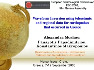
1. European Seismological Commission ESC 2008, 31st General Assembly Waveform Inversion using teleseismic and regional data for earthquakes that occurred in Greece Alexandra Moshou, Panayotis Papadimitriou, Konstantinos Makropoulos Hersonissos, Crete, Greece, 7-12 September 2008

2. Main task of this study Determination of Seismic parameters of an earthquake • Seismic Moment Tensor, Mij • Seismic source • Depth • Magnitude, M0 Methodology Body wave modeling and regional modeling by calculation synthetics seismograms and fitting with the corresponding observed

3. Teleseismic Data Regional – Local Data Global Seismological Network Unified Seismological Network 30°<Δ<90° Δ<6° Eigenvaluesand eigenvectors analysis Jost and Hermann (1988) Descrete wavenumber technique Bouchon (1981, 2002), Zahradnik (2003) Deconvolution of instrument response ~ application of band passed filtered Preparation of data 0.01– 0.1 Hzsampling rate 0.25 sample/sec 0.01 – 0.1 Hzsampling rate 0.25 sample/sec

4. Global Seismological Network TELESEISMIC • Hellenic Seismological Network • Mednet • Geofon LOCAL – REGIONAL Preparation of data STEP 1: SELECTION OF DATA DATA

5. 5 Green’ s function elementary focal mechanisms – linear combination TELE LOCAL REGIONAL Axitra code (Bouchon, 1981) Zahradnik et al. (2003) Preparation of data STEP 2: SYNTHETICS SEISMOGRAMS SYNTHETICS STEP 3: DECONVOLUTION – FILTERED • Deconvolution of instrument response and band passed filtered between 0.01 – 0.1 Hz • Inversion of the selected waveforms

6. Calculationof synthetic seismograms ρ :the density at the source c: the velocity of P, S-waves g(Δ,h) : geometric spreading r0 : the radius of the earth Ri : the radiation pattern in case of P, SH, SV-waves (i=1, 2, 3) respectively the moment rate

7. Elementary moment tensors

8. Forward problem • d : a vector of length m, which corresponds the observed displacements • G : a non – square matrix, with dimensions mxn, whose elements are a set of five elementary Green’s functions • m : a vector of length n, which corresponds the moment tensor elements determination the parameters of the model by the method of trial and error

9. Inverse problem • d : m x 1 matrix," lives” in data – space of n – components, represents the observed data set • G : non - square m x n matrix, green’s function • m : n x 1 vector, the model vector m “lives” in model – space of m – components determination The source parameters using numerical methods

10. Moment Tensor Inversion where a1,…,a5 are the components of the model m

11. Moment Tensor Inversion • n < 5 : under – determined system • n > 5 : over – determinedsystem G non – square matrix pseudo inverse GTG = square matrix

12. The Linear Least Squares Problem • In general, Ax = b with m > n has no solution • Instead, try to minimize the residual r = b − Ax • With the 2-norm we obtain the linear least squares problem (LSP): LINEAR LEAST SQUARES PROBLEM Given Amxn , m>n find x such that:

13. Matrix Decompositions

14. QR - factorization Least – Square method 1: QR - Factorization where: QR – factorization transform the least – square problem into a triangular least - square

15. Least – Square method 1: QR - Factorization Algorithm • QR factorization of G, G = Q·R • form d = QT·b • solve R·x = d , backward substitution 2·m·n2 (flops) 2·m·n (flops) n2 (flops) Total flops: 2·m·n2 (flops)

16. Methods for QR - Factorization • Householder transformations (elementary reflectors) • Givens transformations (plane rotations) • Gram – Schmidt orthogonalization

17. QR – Householder Reflections • Householder transformationshas form where v is nonzero vector • From definition, H = HT = H-1, so H is both orthogonal • and symmetric • For given vector b, choose v so that

18. QR – Householder Reflections

19. Least – Square method 2: CHOLESKY - NORMAL EQUATIONS G: positive matrix H: upper triangular matrix Cholesky factor Then we solve the two triangular system by the back – substitution

20. method 1 has better numerical properties, method 2 is faster Least – Square method 2: CHOLESKY - NORMAL EQUATIONS Algorithm • calculate C = GT G (C is symmetric) • Cholesky factorization C = HHT • calculate y = H·m • solve H·m = b by forward substitution • solve HT·m = y by backward substitution Total flops:

21. ALL MATRICES HAVE A SINGULAR VALUE DECOMPOSITION SINGULAR VALUE DECOMPOSITION We’d like to more formally introduce you to Singular Value Decomposition (SVD) and some of its applications SVD is a type of factorization for a rectangular real or complex matrix

22. Singular value decomposition Any real matrix G (mxn) can be decomposed in three parts U, V, L where : • U,V : n x n, m x m orthogonal matrices respectively • The columns of U,V are the eigenvectors , respectively • Λ : unique n x m diagonal matrix, with real and non – negative • elements λi ,(singular values of G) i = 1,2, …, min (m, n) > 0, in order :

23. Singular Value Decomposition • U, V : orthogonal matrices (nxn) and (mxm) corresponding, which elements are the eigenvectors of the matrices GTG and GGT respectively. • Λ : diagonal matrix, (nxm) which element, σi are the singular values of the GTG or GGT The singular values σi [i=1, 2, …, min(m,n)] are real, non – zero and non – negative,

24. Quality of the solution CONDITION NUMBER ERROR λ,μ : max. and min. eigenvalue ATA k(A) >> unstable k(A) << stable

25. Applications • Leonidio earthquake 2008/01/08 Teleseismic distances • Methoni earthquake 2008/02/14 • Andravida earthquake 2008/06/08 Rodos earthquake 2008/07/15 20080204 20080625 Regional – local distances 20080608 20080715 • Patras sequence 2008/02/04 20080214 20080106 20080612 Crete earthquake 2008/06/12 Atalanti earthquake 2008/06/25

26. The January 6, 2008 Leonidio earthquake Mw = 6.0 (37.120 Ν, 22.770 Ε) Deep event d=85 km Red = observed waveforms Blue = synthetics waveforms

27. The January 8, 2008 Leonidio earthquake Mw= 6.0 ~ inversion Stations at epicentral distances 30°<Δ<90° D.C=98% CLVD=2% Stations at regional distances Δ<6°

28. The February 14, 2008 Methoni (12:09) earthquake Mw = 6.0 (36. 340 Ν, 21.920 Ε) Shallow event d=24 km Red = observed waveforms Blue = synthetics waveforms

29. The February 14, 2008 Methoni (12:09) earthquake Mw = 6.0 ~ inversion Stations at epicentral distances 30°<Δ<90° D.C=87% CLVD=13% Stations at regional distances Δ<6° D.C=78% CLVD=22%

30. The June 6, 2008 Andravida earthquake Mw= 6.4 37.94°Ν21.51°Ε shallow event d=15 km Red = observed waveforms Blue = synthetics waveforms

31. The June 6, 2008 Andravida earthquake Mw = 6.4 ~ inversion Stations at epicentral distances 30°<Δ<90° D.C = 95 % CLVD = 5% Stations at local distances

32. The July 15, 2008 Rodos earthquake Mw = 6.4 Stations at epicentral distances 30°<Δ<90° Stations at regional distances Δ<6°

33. 04 February 2008 (GMT 20:25) 04 February 2008 (GMT 22:15) The sequence of February 4, 2008 Patras (GMT 20:25, 22:15) earthquake Mw = 4.7 and Mw = 4.5

34. The June 12, 2008 Crete earthquake Mw = 5.0 34.96°Ν26.26°Ε d=20 km Red = observed waveforms Blue = synthetics waveforms

35. The June 25, 2008 Atalanti earthquake, MW = 4.5 38.71°Ν22.81°Ε d=15 km Red = observed waveforms Blue = synthetics waveforms

36. Moment tensor solutions Forward – InversionProblem

37. Conclusions • It has developed a new procedure based upon the moment tensor inversion, to obtain the source parameters of an earthquake, taking to account a specific depth. • This methodology is based in numerical methods, QR decomposition, Cholesky decomposition via normal equations and singular value decomposition • The method of Singular Value Decomposition is based in the eigenvalues and eigenvectors of the matrix (GTG) or (GGT). For this reason this method is more stable than others, QR is more stable while Cholesky is faster. • In all the applications the Singular Value Decomposition give up to 90% Double Couple and a very good fit between observed and synthetics seismograms. • Our solution was compared with others than proposed from others institutes and it was in very good agreement.

38. THE END THANK YOU FOR YOUR ATTENTION