Chapter 4: Divide and Conquer
The Design and Analysis of Algorithms. Chapter 4: Divide and Conquer. Chapter 4. Divide and Conquer Algorithms. Basic Idea Merge Sort Quick Sort Binary Search Binary Tree Algorithms Closest Pair and Quickhull Conclusion. Basic Idea.


Chapter 4: Divide and Conquer
E N D
Presentation Transcript
The Design and Analysis of Algorithms Chapter 4:Divide and Conquer
Chapter 4. Divide and Conquer Algorithms • Basic Idea • Merge Sort • Quick Sort • Binary Search • Binary Tree Algorithms • Closest Pair and Quickhull • Conclusion
Basic Idea • Divide instance of problem into two or more smaller instances • Solve smaller instances recursively • Obtain solution to original (larger) instance by combining these solutions
a problem of size n subproblem 1 of size n/2 subproblem 2 of size n/2 a solution to subproblem 1 a solution to subproblem 2 a solution to the original problem Basic Idea
General Divide-and-Conquer Recurrence T(n) = aT(n/b) + f (n)where f(n)(nd), d 0 Master Theorem:If a < bd, T(n) (nd) If a = bd, T(n) (nd log n) If a > bd, T(n) (nlog b a ) • Examples: T(n) = T(n/2) + nT(n) (n ) Here a = 1, b = 2, d = 1, a < bd T(n) = 2T(n/2) + 1T(n) (nlog 2 2) = (n ) Here a = 2, b = 2, d = 0, a > bd
Examples • T(n) = T(n/2) + 1T(n) (log(n) ) Here a = 1, b = 2, d = 0, a = bd • T(n) = 4T(n/2) + nT(n) (n log 2 4)= (n 2) Here a = 4, b = 2, d = 1, a > bd • T(n) = 4T(n/2) + n2T(n) (n2 log n) Here a = 4, b = 2, d = 2, a = bd • T(n) = 4T(n/2) + n3T(n) (n3) Here a = 4, b = 2, d = 3, a < bd
Mergesort • Split array A[0..n-1] in two about equal halves and make copies of each half in arrays B and C • Sort arrays B and C recursively • Merge sorted arrays B and C into array A
Analysis of Mergesort • All cases have same efficiency: Θ(n log n) • Number of comparisons in the worst case is close to theoretical minimum for comparison-based sorting: log2n!≈n log2 n - 1.44n • Space requirement: Θ(n) (not in-place) • Can be implemented without recursion (bottom-up)
p Quicksort • Select a pivot (partitioning element) – here, the first element • Rearrange the list so that all the elements in the first s positions are smaller than or equal to the pivot and all the elements in the remaining n-spositions are larger than or equal to the pivot (see next slide for an algorithm) • Exchange the pivot with the last element in the first (i.e., ) sub-array — the pivot is now in its final position • Sort the two sub-arrays recursively A[i]p A[i]p
Analysis of Quicksort • Best case: split in the middle — Θ(n log n) • Worst case: sorted array — Θ(n2) • Average case: random arrays — Θ(n log n) • Improvements: • better pivot selection: median of three partitioning • switch to insertion sort on small subfiles • elimination of recursion • Quicksort is considered the method of choice for internal sorting of large files (n ≥ 10000)
Binary Search • Very efficient algorithm for searching in sorted array: K vs A[0] . . . A[m] . . . A[n-1] • If K = A[m], stop (successful search); • otherwise, continue searching by the same method in A[0..m-1] if K < A[m], and in A[m+1..n-1] if K > A[m]
Analysis of Binary Search • Time efficiency Worst-case recurrence: Cw (n) = 1 + Cw( n/2 ), Cw (1) = 1 solution: Cw(n) =log2(n+1) • Optimal for searching a sorted array • Limitations: must be a sorted array (not linked list)
Binary Tree Algorithms • Binary tree is a divide-and-conquer ready structure Ex. 1: Classic traversals (preorder, inorder, postorder) • Algorithm Inorder(T) if T Inorder(Tleft) print(root of T) Inorder(Tright) • Efficiency: Θ(n)
Binary Tree Algorithms Ex. 2: Computing the height of a binary tree h(T) = max{ h(TL), h(TR) } + 1 if T and h() = -1 Efficiency: Θ(n)
Closest Pair Problem Step 1: Divide the points given into two subsets S1 and S2 by a vertical line x = c so that half the points lie to the left or on the line and half the points lie to the right or on the line.
Closest Pair Problem • Step 2Find recursively the closest pairs for the left and right subsets. • Step 3Set d = min {d1, d2} Let C1 and C2 be the subsets of points in the left subset S1 and of the right subset S2, respectively, that lie in this vertical strip. The points in C1 and C2 are stored in increasing order of their y coordinates, which is maintained by merging during the execution of the next step. • Step 4For every point P(x,y) in C1, we inspect points in C2 that may be closer to P than d. There can be no more than 6 such points (because d ≤ d2)
Closest Pair Problem • The worst case scenario is depicted below
Efficiency of the Closest Pair Problem Running time of the algorithm T(n) = 2T(n/2) + M(n), where M(n) O(n) By the Master Theorem (with a = 2, b = 2, d = 1) T(n) O(n log n)
Quickhull Algorithm Convex hull: smallest convex set that includes given points • Assume points are sorted by x- coordinate values • Identify extreme pointsP1 and P2 (leftmost and rightmost) • Compute upper hull recursively: • find point P max that is farthest away from line P1P2 • compute the upper hull of the points to the left of line P1Pmax • compute the upper hull of the points to the left of line PmaxP2 • Compute lower hull in a similar manner
Pmax P2 P1 Quickhull Algorithm
Efficiency of Quickhull Algorithm Finding point farthest away from line P1P2 can be done in linear time • Time efficiency: • worst case: Θ(n2) (as quicksort) • average case: Θ(n ) (under reasonable assumptions about distribution of points given) • If points are not initially sorted by x-coordinate value, this can be accomplished in O(n log n) time
Conclusion • Very efficient solutions. • It is the choice when the following is true: • the problem can be described recursively - in terms of smaller instances of the same problem. • the problem-solving process can be described recursively, i.e. we can combine the solutions of the smaller instances to obtain the solution of the original problem Note that we assume that the problem is split in at least two parts of equal size, not simply decreased by a constant factor.