Download
1 / 24
240 likes | 256 Vues
Explore the different models of computation, including Turing Machines and Finite State Machines, and how they can be used to solve complex problems. Discover the significance of complexity classes and the importance of modeling input, output, and processing in a computer.

E N D
Class 30: Models of Computation David Evans http://www.cs.virginia.edu/evans CS200: Computer Science University of Virginia Computer Science
Menu • Are complexity classes really meaningful? • How can we model computation? • Turing Machines • Universal Turing Machine CS 200 Spring 2003
Complexity Classes • We claimed problem complexity doesn’t depend on the language or computer: problems are in class P and NP regardless of what kind of computer you have • In PS7, we saw that if you have a quantum computer you solve a problem that has no known polynomial time solution on a “normal computer” in polynomial time. • This should bother you! CS 200 Spring 2003
How should we model a Computer? Colossus (1944) Cray-1 (1976) Apollo Guidance Computer (1969) IBM 5100 (1975)
Modeling Computers • Input • Without it, we can’t describe a problem • Output • Without it, we can’t get an answer • Processing • Need some way of getting from the input to the output • Memory • Need to keep track of what we are doing CS 200 Spring 2003
Modeling Input Punch Cards Altair BASIC Paper Tape, 1976 Engelbart’s mouse and keypad CS 200 Spring 2003
Simplest Input • Non-interactive: like punch cards and paper tape • One-dimensional: just a single tape of values, pointer to one square on tape 0 0 1 1 0 0 1 0 0 0 How long should the tape be? Infinitely long! We are modeling a computer, not building one. Our model should not have silly practical limitations (like a real computer does). CS 200 Spring 2003
Modeling Output • Blinking lights are cool, but hard to model • Output is what is written on the tape at the end of a computation Connection Machine CM-5, 1993 CS 200 Spring 2003
Modeling Processing • Evaluation Rules • Given an input on our tape, how do we evaluate to produce the output • What do we need: • Read what is on the tape at the current square • Move the tape one square in either direction • Write into the current square 0 0 1 1 0 0 1 0 0 0 Is that enough to model a computer? CS 200 Spring 2003
Modeling Processing • Read, write and move is not enough • We also need to keep track of what we are doing: • How do we know whether to read, write or move at each step? • How do we know when we’re done? • What do we need for this? CS 200 Spring 2003
Finite State Machines 1 0 0 2 1 Start 1 # HALT CS 200 Spring 2003
Hmmm…maybe we don’t need those infinite tapes after all? not a paren not a paren ( 2 1 Start ) ) What if the next input symbol is ( in state 2? # HALT ERROR CS 200 Spring 2003
How many states do we need? not a paren not a paren ( 2 not a paren 1 Start ( ) 3 ) not a paren ) # ( 4 HALT ERROR ) ( CS 200 Spring 2003
Finite State Machine • There are lots of things we can’t compute with only a finite number of states • Solutions: • Infinite State Machine • Hard to describe and draw • Add a tape to the Finite State Machine CS 200 Spring 2003
FSM + Infinite Tape • Start: • FSM in Start State • Input on Infinite Tape • Pointer to start of input • Move: • Read one input symbol from tape • Follow transition rule from current state • To next state • Write symbol on tape, and move L or R one square • Finish: • Transition to halt state CS 200 Spring 2003
Matching Parentheses • Repeat until halt: • Find the leftmost ) • If you don’t find one, the parentheses match, write a 1 at the tape head and halt. • Replace it with an X • Look left for the first ( • If you find it, replace it with an X (they matched) • If you don’t find it, the parentheses didn’t match – end write a 0 at the tape head and halt CS 200 Spring 2003
Matching Parentheses Input: ) Write: X Move: L ), X, L (, (, R X, X, L X, X, R 2: look for ( 1 Start (, X, R #, 0, # #, 1, # HALT Will this report the correct result for (()? CS 200 Spring 2003
Matching Parentheses (, (, R X, X, L ), X, L X, X, R 1 2: look for ( (, X, R Start #, #, L #, 1, # #, 0, # 3: look for ( X, X, L HALT #, 1, # (, 0, # CS 200 Spring 2003
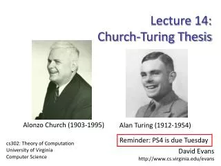
Turing Machine • Alan Turing, On computable numbers: With an application to the Entscheidungsproblem, 1936 • Turing developed the machine abstraction to show the halting problem really leads to a contradiction • Our informal argument, depended on assuming we could do if and everything else except halts? CS 200 Spring 2003
Describing Turing Machines z z z z z z z z z z z z z z z z z z z z z z TuringMachine ::= < Alphabet, Tape, FSM > Alphabet ::= { Symbol* } Tape ::= < LeftSide, Current, RightSide > OneSquare ::= Symbol | # Current ::= OneSquare LeftSide ::= [ Square* ] RightSide ::= [ Square* ] Everything to left of LeftSide is #. Everything to right of RightSide is #. ), X, L ), #, R (, #, L 2: look for ( 1 Start (, X, R HALT #, 0, - #, 1, - Finite State Machine CS 200 Spring 2003
), X, L ), #, R (, #, L Describing Finite State Machines 2: look for ( 1 Start (, X, R #, 0, # #, 1, # HALT TuringMachine ::= < Alphabet, Tape, FSM > FSM ::= < States, TransitionRules, InitialState, HaltingStates > States ::= { StateName* } InitialState ::= StateName must be element of States HaltingStates ::= { StateName* } all must be elements of States TransitionRules ::= { TransitionRule* } TransitionRule ::= < StateName, ;; Current State OneSquare, ;; Current square StateName, ;; Next State OneSquare, ;; Write on tape Direction > ;; Move tape Direction ::= L, R, # Transition Rule is a procedure: StateName X OneSquare StateName X OneSquare X Direction CS 200 Spring 2003
), X, L ), #, R (, #, L Example Turing Machine 2: look for ( 1 Start (, X, R #, 0, # #, 1, # HALT TuringMachine ::= < Alphabet, Tape, FSM > FSM ::= < States, TransitionRules, InitialState, HaltingStates > Alphabet ::= { (, ), X } States ::= { 1, 2, HALT } InitialState ::= 1 HaltingStates ::= { HALT} TransitionRules ::= { <1, ), 2, X, L >, < 1, #, HALT, 1, # >, < 1, ), #, R >, < 2, (, 1, X, R >, < 2, #, HALT, 0, # >, < 2, ), #, L >,} CS 200 Spring 2003
Enumerating Turing Machines • Now that we’ve decided how to describe Turing Machines, we can number them • TM-5023582376 = balancing parens • TM-57239683 = even number of 1s • TM-3523796834721038296738259873 = Photomosaic Program • TM-3672349872381692309875823987609823712347823 = WindowsXP Not the real numbers – they would be much bigger! CS 200 Spring 2003
Charge • Friday, next week: • Lambda Calculus model of computation • Very different from Turing Machines, but we will show that it is exactly as powerful! • Design reviews: sign up today! CS 200 Spring 2003