Wireless, Mobile, Ad-Hoc Network Routing
Wireless, Mobile, Ad-Hoc Network Routing. Mario Gerla, UCLA CSD FOCUS 99. Outline: What is an Ad-Hoc Wireless Network The wireless routing challenge Review of proposed solutions (Distance Vector, Link State, On-Demand, Location Based) Simulation test bed Performance results.


Wireless, Mobile, Ad-Hoc Network Routing
E N D
Presentation Transcript
Wireless, Mobile, Ad-Hoc Network Routing Mario Gerla, UCLA CSD FOCUS 99
Outline: • What is an Ad-Hoc Wireless Network • The wireless routing challenge • Review of proposed solutions (Distance Vector, Link State, On-Demand, Location Based) • Simulation test bed • Performance results
Cellular vs Multihop Standard Base-Station Cellular Networks Instant Infrastructure, Multihop wireless Networks
Ad-Hoc Network Characteristics • Instantly deployable, reconfigurable infrastructure • Node mobility • Heterogeneous nodes (big/small; fast/slow etc) • Heterogeneous traffic (voice, image, video, data) • Limited battery power • Multihopping ( to save power, overcome obstacles, enhance spatial spectrum reuse, etc.)
Ad-Hoc Network Applications • Disaster Recovery (flood, fire, earthquakes etc) • Law enforcement (crowd control, border patrol etc) • Search and rescue in remote areas • Sport events, festivals • Ad hoc nomadic, collaborative computing • Indoor network appliances • Sensor networks • Battlefield
Wireless multihop routing challenges • mobility • need to scale to large numbers (1000's) • unreliable radio channel (fading etc) • limited bandwidth • limited power • need to support multimedia (QoS)
Proposed Routing Approaches • Conventional wired-type schemes (global routing, proactive): • Distance Vector; Link State • Hierarchical (global routing) schemes: • Fisheye, Hierarchical State Routing • On - Demand, reactive routing: • Source routing; backward learning • Location Assisted routing (Geo-routing): • DREAM, LAR etc
Conventional wired routing limitations • Distance Vector (eg, Bellman-Ford): • routing control O/H linarly increasing with net size • convergence problems (count to infinity); potential loops • Link State (eg, OSPF): • link update flooding O/H caused by frequent topology changes CONVENTIONAL ROUTING DOES NOT SCALE TO SIZE AND MOBILITY
Distance Vector 0 Routing table at node 5 : 1 3 2 4 5
1 Link State Routing • At node 5, based on the link state packet, topology table is constructed: • Dijkstra’s Algorithm can then be used for the shortest path 0 {1} {0,2,3} {1,4} 3 2 {1,4,5} 4 {2,3,5} 5 {2,4}
REMEDY #1: use hierarchical routing to reduce table size and table update overhead Proposed hierarchical schemes: • Fisheye (implicit hierarchy induced by "scope") • Hierarchical State Routing • Zone routing (hybrid scheme)
Fisheye State Routing • Topology based routing • similar to link state (e.g., OSPF) • Routing information is periodically exchanged with neighbors only • similar to distance vector • Routing update frequency decreases with distance to destination • Higher frequency updates within a close zone and lower frequency updates to a remote zone • Highly accurate routing information about the immediate neighborhood of a node; progressively less detail for areas further away from the node
2 8 3 5 9 1 9 4 6 Hop=1 7 10 12 13 Hop=2 19 18 21 11 Hop>2 15 22 36 14 23 17 16 20 29 35 27 25 24 26 28 34 30 32 31 Scope of Fisheye
Message Reduction in FSR LST HOP 0 LST HOP 0:{1} 1:{0,2,3} 2:{5,1,4} 3:{1,4} 4:{5,2,3} 5:{2,4} 1 0 1 1 2 2 0:{1} 1:{0,2,3} 2:{5,1,4} 3:{1,4} 4:{5,2,3} 5:{2,4} 2 1 2 0 1 2 1 3 LST HOP 2 0:{1} 1:{0,2,3} 2:{5,1,4} 3:{1,4} 4:{5,2,3} 5:{2,4} 2 2 1 1 0 1 4 5
Hierarchical State Routing (HSR) • Main challenge: maintain/update the hierarchical partitions in the face of mobility • Solution: distinguish between “physical” partitions and “logical” grouping • physical partitions are based on geographical proximity • logical grouping is based on functional affinity between nodes (e.g., tanks of same battalion, students of same class) • Physical partitions enable reduction of routing overhead • Logical groupings enable efficient location management strategies using Home Agent concepts
3 1 Level = 2 2 3 1 Level = 1 4 2 8 9 6 3 1 Level = 0 10 11 7 5 4 HSR - physical multilevel partitions HSR table at node 5: DestID 1 6 7 <1-2-> <1-4-> <3--> Path 5-1 5-1-6 5-7 5-1-6 5-7 5-7 HID(5): <1-1-5> HID(6): <3-2-6> Hierarchical addresses (MAC addresses)
HSR - logical partitions and location management • Logical (IP like) type address <subnet,host> • Each subnet corresponds to a particular user group (e.g., tank battalion in the battlefield, search team in a search and rescue operation, etc) • logical subnet spans several physical clusters • Nodes in same subnet tend to have common mobility characteristic (i.e., locality) • logical address is totally distinct from MAC address
HSR - logical partitions and location management (cont’d) • Each subnetwork has at least one Home Agent to manage membership • Each member of the subnet registers its own hierarchical address with Home Agent • periodically/event driven registration; stale addresses are timed out by Home Agent • Home Agent hierarchical addresses propagated via routing tables; or queried at a Name Server
On-Demand Routing Protocols • Routes are established “on demand” as requested by the source • Only the active routes are maintained by each node • Channel/Memory overhead is minimized • Two leading methods for route discovery: source routing and backward learning (similar to LAN interconnection routing)
Existing On-Demand Protocols • Dynamic Source Routing (DSR) • Associativity-Based Routing (ABR) • Ad-hoc On-demand Distance Vector (AODV) • Temporarily Ordered Routing Algorithm (TORA) • Zone Routing Protocol (ZRP) • Signal Stability Based Adaptive Routing (SSA)
Dynamic Source Routing (DSR) • Uses source routing instead of hop-by-hop routing • No periodic routing update message is sent • Nodes ignore topology changes not affecting active routes with packets in the pipe • The first path discovered is selected as the route • Two main phases • Route Discovery • Route Maintenance
DSR - Route Discovery • To establish a route, the source floods a Route Request message with a unique request ID • Route Reply message containing path information is sent back to the source either by • the destination, or • intermediate nodes that have a route to the destination • Each node maintains a Route Cache which records routes it has learned and overheard over time
Performance Evaluation Enviroment • PARSEC simulation enviroment • 100 nodes • 1000mx1000m square area • transmission range: 100m • channel data rate: 2 Mbps • random mobility model • UDP traffic between randomly selected node pairs • cluster-token MAC layer protocol • HSR • 2 level physical partition • 1 level logical groupings, number of logical subnets varies with network size • FSR • 2 level fisheye scoping • fisheye radius is 2 hops
DSR - Route Maintenance • Route maintenance performed only while route is in use • Monitors the validity of existing routes by passively listening to acknowledgments of data packets transmitted to neighboring nodes • When problem detected, send Route Error packet to original sender to perform new route discovery
Location-Aided Routing • Ko and Vaidya (Texas A & M) • Location assisted (requires GPS) • On-demand • No periodic messages • Works similar to DSR except LAR limits the flooded area of Route Requests using location information
LAR (cont’d) • Scheme 1 • The source specifies a request zone which includes the source and the area where the destination may reside • Nodes within the request zone propagate Route Requests • Scheme 2 • The source specifies the distance between itself and the destination • Nodes forward Route Requests if their distances to the destination is less than or equal to the distance indicated by the packet
DREAM • Basagni, et al. (U of Texas, Dallas) • Location assisted (requires GPS) • Coordinates of each node are recorded in the route table instead of route vectors • Distance Effect: Send location updates to nearby nodes more frequently • Location update frequencies are adjusted to mobility rate
DREAM (cont’d) • The source partially floods data to nodes that are in the direction of the destination • The source specifies possible next hops in the data header using location information • Next hop nodes select their own list of next hops and include the list into data header • If the source finds no neighbors in the direction of the destination or has no fresh location information of the destination, data is flooded to the entire network
Application Processing Application Setup Application RTP Wrapper RCTP Transport Wrapper TCP/UDP Control Transport RSVP IP Wrapper IP IP/Mobile IP Routing VC Handle Flow Control Routing Clustering Packet Store/Forward Network Link Layer Packet Store/Forward Ack/Flow Control Clustering MAC Layer Frame Wrapper RTS/CTS CS/Radio Setup Frame Processing Radio Status/Setup Radio Propagation Model Mobility Channel GloMoSim Simulation Layers Control Plane Data Plane
Location Based Routing Simulation (LAR and DREAM) • 50 nodes; 750m X 750 m space • Free space channel propagation model • Radio with capture ability • MAC: IEEE 802.11 DCF • 10 UDP data sessions with constant bit rate
Simulation Results • Number of data packets transmitted per data packet delivered
Simulation Results (cont’d) • Number of control bytes transmitted per data byte delivered
Simulation Results (cont’d) • Packet delivery ratio
Conclusions • Conventional (wired net) routing schemes suffer of O/H, mobility and scalability limitations • Hierarchical routing reduces O/H and improves scalability (at the expense of accuracy). • On Demand routing eliminates background routing control O/H. It introduces latency; it does not support QoS routing
Conclusions (cont’d) • Location assisted routing can enhance performance in both on demand (LAR) and table driven (DREAM) settings; GPS required. • No routing scheme works best in all situations; selection must be guided by application scenario • Open problem: efficient location management and resource discovery in highly mobile environment