2-D Trees
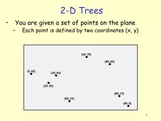
2-D Trees. You are given a set of points on the plane Each point is defined by two coordinates (x, y). (60,75). (80,65). (5,45). (35,40). (25,35). (85,15). (50,10). (90,5). 2-D Trees.

2-D Trees
E N D
Presentation Transcript
2-D Trees • You are given a set of points on the plane • Each point is defined by two coordinates (x, y) (60,75) (80,65) (5,45) (35,40) (25,35) (85,15) (50,10) (90,5)
2-D Trees • The problem is to design a Data Structure that would store these points and perform the following operations efficiently • Insert - a point into the set • Delete - an existing point from the set • Point Query – given a point, see if it exists in the set • Range Query – find all points that fall into a • rectangular region • Nearest Neighbor Query – Find the point that is • closest to a given query point
Flashback: 1-D Search Trees • Recall our 1-D search trees • BST, AVL, Splay, B-Tree … • The problem there was to manipulate keys that lay over a single axis (thus the name 1-D tree) • Our search trees worked by cutting this axis at a key point, thus dividing the keys into 2 sets: (1) those smaller than the key, (2) those bigger than the key • Here is an example 60 5 25 35 50 85 90 80
1-D Search Trees – BST Example <50 >50 <25 >25 <80 >80 <5 >5 <35 >35 <60 >60 >90 <90 60 5 25 35 50 90 80 50 25 80 35 5 60 90
2-D Trees • Extension to 2-D trees uses the same idea • At one level, cut the plane perpendicular to one axis, at the next level, cut it perpendicular to the other • Arrival order of the points: • (50,10) (25,35) (80,65) (5,45) (60,75) (35,40) (90,5) (85,15) (50,65) (60,75) (50,65) (80,65) (5,45) (35,40) (25,35) (85,15) (90,5) (50,10)
Example 2-D Tree (60,75) (50,65) (80,65) (5,45) (35,40) root (25,35) x (50,10) y (80,65) (25,35) (85,15) y (90,5) x (5,45) x (60,75) (90,5) x (50,10) y (35,40) (85,15) (50,65) y y
2-D Tree Ops – Point Query root // axis: 0 means x-axis, 1 means y-axis TreeNode *Find(TreeNode *t, Point p, int axis){ if (t == NULL) return NULL; if (t->p equals p) return t; if (axis == 0){ if (p.x < t->p.x) returnFind(t->left, p, 1); else returnFind(t->right, p, 1); //>= } else { if (p.y < t->p.y) returnFind(t->left, p, 0); else returnFind(t->right, p, 0); //>= } //end-else } /* end-Find */ x (50,10) y (25,35) (80,65) x (5,45) (90,5) (60,75) y (35,40) (85,15) (50,65) structPoint {int x, y;} structTreeNode { Point p; TreeNode *left, *right; }; TreeNode *root = NULL;
Iterative 2-D Tree Point Query TreeNode *Find(TreeNode *t, Point p){ int axis = 0; // Initial axis while (t != NULL){ if (t.p equals p) return t; if (axis == 0){ if (p.x < t->p.x) t = t->left; else t = t->right; // >= } else { if (p.y < t->p.y) t = t->left; else t = t->right; // >= } // end-else axis = !axis; // change the axis } // end-while return NULL; } /* end-Find */
2-D Tree Insert(Point p) z • Create a new node “z” and initialize it with the point to insert • E.g.: Insert (95, 80) • Then, begin at the root and trace a path down the tree as if we are searching for the node that contains the point • The new node must be a child of the node where we stop the search (95,80) NULL NULL Node “z” to be inserted z->p = (95, 80) root x (50,10) y (25,35) (80,65) x (5,45) (90,5) (60,75) y (35,40) (85,15) (50,65) (95,80) After (95,80) is inserted
2-D Tree Insert point (95,80) (95,80) (60,75) (50,65) (80,65) root (5,45) root (35,40) (25,35) x (50,10) y (25,35) (80,65) (85,15) (95,80) (90,5) x (5,45) (90,5) (60,75) (50,10) y (35,40) (85,15) (50,65)
2-D Tree Ops – Insert void Insert(TreeNode *t, Point p){ int axis = 0; // Initial axis TreeNode *z = new TreeNode(p); while (t){ if (t.p equals p){return; /* duplicate point */} if (axis == 0){ if (p.x < t->p.x){ if (!t->left){t->left = z; return;} else t = t->left; } else { if (!t->right){r->right = z; return;} else t = t->right; } //end-else } else { /* axis = 1, i.e., y axis */ if (p.y < t->p.y){ if (!t->left){t->left = z; return;} else t = t->left; } else { if (!t->right){r->right = z; return;} else t = t->right; } //end-else } // end-else axis = !axis; // change the axis } // end-while } /* end-Insert */
2-D Tree Ops – Recursive Insert // axis: 0 – x axis, 1 – y axis TreeNode *Insert(TreeNode *t, Point p, int axis){ if (t == NULL) t = new TreeNode(p); else if (t->p == p) ; //error: duplicate point else if (axis == 0){ if (p.x < t->p.x) t->left = Insert(t->left, p, 1); else t->right = Insert(t->right, p, 1); } else { if (p.y < t->p.y) t->left = Insert(t->left, p, 0); else t->right = Insert(t->right, p, 0); } //end-else return t; } //end-Insert
2-D Tree Ops – Delete(Point p) • Delete is a bit trickier. 3 cases exist • Node to be deleted has no children (leaf node) • Delete (35,40) • Node to be deleted has 1 child • Delete (90,5) • Node to be deleted has 2 children • Delete (50,10) root x (50,10) y (25,35) (80,65) x (5,45) (90,5) (60,75) y (35,40) (85,15) (50,65) (95,80)
Deletion: Case 1 – Deleting a leaf node root root x x (50,10) (50,10) y y (25,35) (25,35) (80,65) (80,65) x (5,45) x (5,45) (90,5) (90,5) (60,75) (60,75) y (35,40) (85,15) (85,15) (50,65) (50,65) (95,80) (95,80) Deleting (35,40): Simply remove the node and adjust the pointers After (35,40) is deleted
Deletion: Case 2 – A node with one child root root x x (50,10) (50,10) y (25,35) y (80,65) (25,35) (80,65) x (5,45) (85,15) (60,75) x (5,45) (90,5) (60,75) y (35,40) (50,65) y (35,40) (95,80) (85,15) (50,65) (95,80) Is this correct? Deleting (90,5): “Splice out” the node by making a link between its child and its parent NO!
Deletion: Case 3 – Node with 2 children root root x (50,65) x (50,10) y (25,35) (80,65) y (25,35) (80,65) x (5,45) (90,5) (60,75) x (5,45) (90,5) (60,75) y (35,40) (85,15) (50,65) (95,80) y (35,40) (85,15) (50,65) (95,80) Now recursively delete the replacement node (50,65) Deleting (50,10): Find the point with the minimum“x” coordinate in the right subtree, copy its contents to the deleted node. Then recursively delete the replacement node
Deletion - Summary • Leaf node – just delete • Internal node (1 or 2 children) • Find the node with the “minimum” value along the cutting dimension (x or y) in the right subtree. Then recursively delete the replacement node
Deletion – Summary (cont) • What if the right subtree is empty? • Happens if the internal node has 1 left child only • We can find the node with the “maximum” value along the cutting dimension in the left subtree? • But this does not work. Recall that we maintain the invariant that points whose coordinates are equal to the cutting axis are stored in the RIGHT subtree. • If we select the replacement point to be the point with the maximum coordinate from the left subtree, and if there are other points with the same coordinate in this subtree, then we will have violated our invariant!
Deletion – Summary (cont) • How do we delete a node with 1 left child then? • The idea is to find the “minimum” point in the left subtree, copy it to the deleted node • Then, move the left subtree over to the right so that it becomes the right child of the deleted node. • The left child is then set to NULL
Deletion Example root root x x (50,30) (35,60) y y (20,45) (20,45) (60,80) (60,80) x x (10,35) (10,35) (80,40) (80,40) y y (20,20) (50,30) (90,60) (20,20) (50,30) (90,60) (70,20) x (70,20) x Delete (35,60) y y (60,10) (60,10) Copy data inside the replacement node (50,30) to the deleted node Find replacement: (50,30) Now, recursively delete the replacement node: (50,30)
Deletion Example (cont) root root x (50,30) x (50,30) y (20,45) (60,80) y (20,45) (60,80) x (10,35) (80,40) x (10,35) (80,40) y (20,20) (60,10) (90,60) y (20,20) (50,30) (90,60) (70,20) x (70,20) x Delete (50,30) y (60,10) y (60,10) Copy data inside the replacement node (60,10) to the deleted node, and move the left subtree over to the right No right child Find the minimum in the left subtree: (60, 10) Now, recursively delete the replacement node: (60,10)
FindMin // Returns the point having the minimum value along // “minAxis” in the tree pointed to by “t” Point *findMin(TreeNode *t, intminAxis, int axis){ if (t == NULL) return NULL; else if (minAxis == axis){ if (t->left == NULL) return &t->p; else return findMin(t->left, minAxis, !axis); } else { TreeNode *p1 = findMin(t->left, minAxis, !axis); TreeNode *p2 = findMin(t->right, minAxis, !axis); return minimum(&t->p, p1, p2, minAxis); } //end-else } //end-findMin
FindMin(t, minaxis = 0, axis = 1); t y (55,40) x (45,20) (35,75) y (30,25) (60,30) (10,65) (70,60) x (15,10) (25,85) (70,15) (20,50) (60,10) (25,15)
2-D Tree Ops - Delete // Deletes point “p” from the tree pointed to by t TreeNode *Delete(TreeNode *t, Point p, int axis){ if (t == NULL) ; // error deleting nonexistent point else if (p equals t->p){ if (t->right != NULL){ // take replacement from right t->p = *(findMin(t->right, axis, !axis); t->right = Delete(t->right, t->p, !axis); } else if (t->left != NULL){ // take replacement from left t->p = *(findMin(t->left, axis, !axis); t->right = Delete(t->left, p, !axis); t->left = NULL; } else t = NULL; } else { ... // typical search code here } //end-else return t; } //end-Delete
2-D Tree Ops – Nearest Neighbor q 16 11 1 5 12 2 7 3 9 10 14 6 15 8 4 13 • Given a query point “q”, find the point closest to “q” • The distance is measured in Euclidean distances, but other sorts of distance measures can easily be integrated
2-D Tree Ops – Nearest Neighbor • The intuitive approach would be to find the leaf node that contains “q”, and then search it and the neighboring cells for closest neighbor • The problem is that the nearest neighbor may be very far away in the sense of the tree’s structure q 16 11 1 5 12 2 7 3 9 10 14 6 15 8 4 13 x 7 y y 9 6 x 14 x 4 1 12 y 15 11 8 y 2 3 Search path x 13 16 x 10 5 Nearest neighbor
2-D Tree Ops – Nearest Neighbor Start at the root & maintain the closest point found so far x 7 Favor branching towards the subtree where “q” is located. Update closest point if possible y y 9 9 6 6 Eliminated x x 12 14 12 14 Eliminated 4 4 1 1 Eliminated y 8 11 8 11 15 15 y 2 2 3 3 x 13 16 13 16 x 10 10 5 5 q 16 11 1 Eliminate braches that are farther away from the closest point found so far. 5 12 2 7 3 Update closest point as 5 9 10 Update closest point as 16 14 6 15 8 4 13
2-D Tree Ops – Nearest Neighbor // Finds the nearest neighbor of a query point “q”. // Initially, c->dist = INFINITY, c->p = (undefined, undefined) void NN(TreeNode*t, int axis, Point q, Rectangle r, Result *c){ if (t == NULL) return; if (distance(q, r) >= c->dist) return; // no overlap. Eliminate int dist = distance(q, t->p); if (dist < c->dist){c->dist = dist; c->p = t->p;} intqv = q->x; intpv = t->p.x; if (axis == 1){qv = q->y; pv = t->p.y;} if (qv < pv){ NN(t->left, !axis, r.trimRight(axis, t->p), c); NN(t->right, !axis, r.trimLeft(axis, t->p), c); } else { NN(t->right, !axis, r.trimLeft(axis, t->p), c); NN(t->left, !axis, r.trimRight(axis, t->p), c); } //end-else } //end-NN
2-D Tree Ops – Nearest Neighbor • The running time of the nearest neighbor searching can be quite bad in the worst case • In particular, it is possible to come up with examples where the search visits every node in the tree, and hence the running time is O(n) • However, the running time can be shown to be much closer to O(logn) where logn is the depth of the tree
2-D Tree Ops – Range Search 16 11 1 5 12 2 7 3 9 10 14 6 15 8 4 13 • The problem is to find (count) all points that fall inside a search region (thus the name range search) • In the given example, the range area is the green rectangle, and points 9, 10 and 12 fall inside this range area
2-D Tree Ops – Range Search 16 11 1 5 12 2 7 3 9 10 14 6 15 8 4 13 x 7 y y 9 6 x 14 x 4 1 12 y 15 11 8 y 2 3 inside range x 13 16 x 10 5 visited
2-D Tree Ops – Range Search // Prints all points that fall inside a range Q // Q is the range area // R is the rectangle covered by the tree pointed to by “t” // Initially R is the whole rectangular area containing ALL points void rangeSearch(TreeNode *t, int axis, RectangleQ, Rectangle R){ if (t == NULL) return; if (Q is disjoint from R) return; if (Q contains t->p) print t->p; rangeSearch(t->left, !axis, Q, R.trimRight(axis, t->p)); rangeSearch(t->right, !axis, Q, R.trimLeft(axis, t->p)); } //end-rangeSearch
K-D Trees • It is possible to easily extend the 2-D trees to higher dimensions • In dimension K>=2, the tree is called a K-D tree • Instead of branching at x or y axis only, we would also branch at other axes (in 3-D, every third level would be branching at the z-axis and so on) • All 2-D tree operations can easily be extended to K-D trees