Download
1 / 44
780 likes | 1.87k Vues
COMSOL Multiphysics Acoustic Transmission Loss Through Periodic Elastic Panels. Courtesy of Anthony Kalinowski, NUWC. Lx. Model Specifications.

E N D
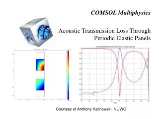
COMSOL MultiphysicsAcoustic Transmission Loss Through Periodic Elastic Panels Courtesy of Anthony Kalinowski, NUWC
Lx Model Specifications • Acoustic transmission loss through elastic panel-like structure which separates two semi-infinite fluids is computed and verified with analytic solutions. The effects of incident angle and frequency are studied. • Important features used: Acoustic-structure interaction with arbitrary incident angle, scattered field formulation, the perfectly matched layer (PML), periodic boundary condition • This model can be extended to model elastic panels which may have complex internal structures, for example, sandwiched honeycomb core. • Presentation layout • Geometry • Meshing • Physical properties and boundary conditions • Postprocessing
Model Description Begin by selecting a 2d geometry without choosing any physics
PML Fluid Steel plate Fluid PML Geometry • 2d geometry using the rectangle/square tool (shift click) • Panel dimension: • 2 inch (thickness) x 2 inch (Lx) • Five subdomains: PML (2), Fluids (2), Elastic Panel (1) (Steel in this model)
Meshing • Mapped Mesh is used • The element distribution can be tuned for each boundary
Adding Physics/Application Modes • Go to Multiphysics -> Model Navigator • Add the three application modes: Plain strain (acpn) Pressure acoustics (acpr) Pressure acoustics (acpr2) • Make sure you use the application modes from the Acoustics Module
Constants/Global Expressions • Constants: 1). Steel data: thickness = 2 inch, Young's modulus = 3e7 psi, Poisson ratio = 0.3, density = 7.2e-4 lb-sec^2/in^4 2). Water data: speed of sound = 5.9e4 in/sec; density 9.6e-5lb-sec^2/in^4 3). Frequency, incident angle, wave number, length • Global expressions: kx, ky, transmission loss, transmitted/reflected pressure
Application Scalar Variables • change the excitation frequencies to freq which was defined as a constant • p_i_acpr = exp(-i*(kx*x+ky*y) [Pa] (incident pressure wave in the incident fluid domain) p_i_acpr2 = 0*exp(-i*(kx*x+ky*y) [Pa] (no incident pressure wave in the tranmitted fluid domain) • Do not check the “Synchronize equivalent variables” box.
Physical properties: Plain Strain • Select the Plain strain from the Multiphysics main menu • Select subdomain 1, 2, 4, 5 and clear the checkbox “Active in the domain” • Select subdomain 3 and enter the steel data defined as constants previously.
Physical properties: Plain Strain • Click Damping tab page and add damping (e.g. Loss factor damping) when necessary • no damping in this model
Boundary Conditions: Plain Strain • Constraints all four steel panel boundaries: free
Boundary Conditions: Plain Strain • Top boundary: enter the pressure load; you can use the global/local tangent and normal coord (global is used here) p_t_acpr*nx_acpr p_t_acpr*ny_acpr • Similar for the bottom boundary Note: p_t_acpr is the predefined total pressure when solving for the scattered field as in this case (see below); nx_acpr are ny_acpr are the normal vector components (pointing outward from the acoustic domain (acpr))
Physical properties: PressureAcoustics (acpr) • Select the pressure acoustics (acpr) from the Multiphysics main menu • Select subdomain 1, 2, 3 and clear the checkbox “Active in the domain” • Select subdomain 4, 5 (the top two subdomains) and enter the water data on the Physics tab page
Physical properties: PressureAcoustics (acpr) • Select subdomain 5 only and click the PML tab page • select the Coordinate direction type, absorbing in y-direction only • Enter 2*pi/abs(ky) for the Scaled PML width edit box
Boundary Conditions: Pressue Acoustics (acpr) • Select the boundaries as shown in the figure on the left, and apply the Neutral boundary conditions NOTE: the p used here in the boundary condition is the scattered field instead of the total pressure
Boundary Conditions: Pressue Acoustics (acpr) • Select the boundary as shown in the figure on the left, and apply the Normal acceleration boundary condition nx_acpn*u_tt_acpn+ny_acpn*v_tt_acpn NOTE: these quantities used are predefined. See Physics>Equation Systems > … or the User’s Guide
Application Physics Properties: Pressue Acoustics (acpr) • Go to the Physics Main menu > Properties • Make sure 1) the analysis type is Time-harmonic 2) Solve for Scattered field NOTE: Total pressure = incident pressure + scattered pressure See Acoustics Module User’s Guide for more information
Physical properties: PressureAcoustics (acpr2) • Select the pressure acoustics (acpr2) from the Multiphysics main menu • Select subdomain 3,4,5 (as shown) and clear the checkbox “Active in the domain” • Select subdomain 1, 2 (the top two subdomains) and enter the water data on the Physics tab page
Physical properties: PressureAcoustics (acpr2) • Select subdomain 1 only and click the PML tab page • select the Coordinate direction type, absorbing in y-direction only • Enter 2*pi/abs(ky) for the Scaled PML width edit box
Boundary Conditions: Pressue Acoustics (acpr) • Select the boundaries as shown in the figure on the left, and apply the Sound hard boundar (wall) boundary conditions NOTE: the p used here in the boundary condition is the total field since we are solving for the total field for the transmitted fluid domain.
Boundary Conditions: Pressue Acoustics (acpr2) • Select the boundary as shown in the figure on the left, and apply the Normal acceleration boundary condition nx_acpn*u_tt_acpn+ny_acpn*v_tt_acpn NOTE: these quantities used are predefined. See Physics>Equation Systems > … or the User’s Guide
Application Physics Properties: Pressue Acoustics (acpr2) • Go to the Physics Main menu > Properties • Make sure 1) the analysis type is Time-harmonic 2) Solve for total field NOTE: The incident pressure wave is zero in the transmitted fluid domain.
Boundary Conditions: Pressue Acoustics (acpr2) • Select the boundary as shown in the figure on the left, and apply the Normal acceleration boundary condition nx_acpn*u_tt_acpn+ny_acpn*v_tt_acpn NOTE: these quantities used are predefined. See Physics>Equation Systems > … or the User’s Guide
Physical properties: PressureAcoustics (acpr2) • Select the pressure acoustics (acpr2) from the Multiphysics main menu • Select subdomain 3,4,5 as shown and clear the checkbox “Active in the domain” • Select subdomain 1, 2 (the top two subdomains) and enter the water data on the Physics tab page
Periodic Boundary Conditions: Plain Strain • Go to the Physics main menu > Periodic boundary conditions • On source tab page, select the source boundary as shown on the left, define two constraints: u, v. The constrains are names pconstr1 and pconstr2 by default.
Periodic Boundary Conditions: Plain Strain • In the same dialog box, click the Destination tab • Select the boundary (shown left) as the destination • Enter the expression u*exp(i*kx*Lx) for constraint pconstr1 • On the source vertices and destination vertices tab pages, select the appropriate vertices • Do the same for constraint pconstr2
Periodic Boundary Conditions: pressure acoustics (acpr) • Similarly we define the constraint for the acoustic application mode • On source tab page, select boundaries shown here, define the constraint for p.
Periodic Boundary Conditions: pressure acoustics (acpr) • In the same dialog box, click the Destination tab • Select destination boundaries as shown on the left, and select the constraint name for p • Enter the expression p*exp(i*kx*Lx) • On the source vertices and destination vertices tab pages, select the appropriate vertices
Periodic Boundary Conditions: pressure acoustics (acpr2) • Similarly we define the constraint for the second acoustic application mode • On source tab page, select boundaries shown here, define the constraint for p2.
Periodic Boundary Conditions: pressure acoustics (acpr2) • In the same dialog box, click the Destination tab • Select destination boundaries as shown on the left, and select the constraint name for p2 • Enter the expression p2*exp(i*kx*Lx) • On the source vertices and destination vertices tab pages, select the appropriate vertices
Solve Settings: sweeping incident angles • Time harmonic analysis • Use the parametric solver to sweep some parameter (incident angle here as shown on the left) • Use the default direct solver UMFPACK for this 2D model
Solve Settings • Select on the checkbox “Use Hermitian transpose of constraint matrix and in symmetry detection” • Click OK • Click Solve button (=)
subdomain expression for pressures • To visualize the pressure (total) in two fluids, we define a subdomain expression In subdomain 4: pr = p _t_acpr In subdomain 2: pr = p_t_acpr2
Postprocessing Total pressure Scattered pressure @ theta ~ 0.8*180/pi ~45
Postprocessing: transmitted and reflected pressure ratios • Use the Global Variable Plot under the Postprocessinc menu to plot the transmitted and reflected presssure ratios, respectively • Select preflective and ptransmitted from the Predefined quantities list, click “>” button • Click “Apply”.
Postprocessing: transmitted and reflected pressure ratios • Blue curve: transmitted pressure ratio • Green curve: Reflected pressure ratio
Postprocessing: transmitted and reflected pressure ratios • Blue curve: transmitted pressure ratio • Red curve: Reflected pressure ratio
Solve Settings: sweeping frequency with theta = 0 • Go to the Options menu > Constants, change the theta equal to zero.
Solve Settings: sweeping frequency with theta = 0 • Change the sweeping parameter to freq • Sweep the frequency from 500 to 1e4 Hz. • Use the default direct solver UMFPACK for this 2D model
Postprocessing: Transmission loss • Use the Global Variable Plot under the Postprocessing menu to plot the transmitted and reflected pressure ratios, respectively • Select TL from the Predefined quantities list, click “>” button • Click “Apply”.
Adding Loss Factor Damping • Select the Plain strain from the Multiphysics main menu • Go to the Physics main menu > subdomain settings • Select the subdomain and click the Damping tab page • Select Loss factor damping and enter 0.5 there.
Solve Settings: sweeping incident angles • Time harmonic analysis • Use the parametric solver to sweep some parameter (incident angle here as shown on the left) • Use the default direct solver UMFPACK for this 2D model
Postprocessing: transmitted and reflected pressure ratios • Blue curve: transmitted pressure ratio • Green curve: Reflected pressure ratio
Reference: S. Dey and J. J. Sirron, Proceedings of IMECE 2006, ASME 2006 Internal Mechanical Engineering Congress & Exposition, Chicago, USA