Download
1 / 20
200 likes | 376 Vues
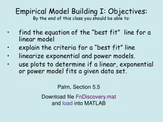
Empirical Model Building Ib: Objectives: By the end of this class you should be able to:. Determine the coefficients for any of the basic two parameter models Plot the data and resulting fits Calculate and describe residuals. Palm, Section 5.5

E N D
Empirical Model Building Ib: Objectives:By the end of this class you should be able to: • Determine the coefficients for any of the basic two parameter models • Plot the data and resulting fits • Calculate and describe residuals Palm, Section 5.5 Download file FnDiscovery.mat and load into MATLAB
1. Below are three graphs of the same dataset. What is the name and equation of the likely model that would match this data?
2. Here are the plots for another dataset. Name the model and write its equation for this case
Fitting a Linear equation via matrices e.g., Fitting the Spring data • Model: y = mx + b • Setup: 1. Design Matrix: >> X = [ones(length(Force),1), Force] 2. Response Vector >> Y= Length • Fit: find the fitted parameters >> B = X \ Y B will be • Predict: calculate predicted y for each x >> Lhat = X*B • Plot: plot the result >> plot(Force, Length, ‘p’, Force, Lhat)(plus labels ...)
A Linear Model & it’s Design Matrix y = b(1) + mx Linear Model: Design Matrix: Matlab Syntax: (to convert a row vector of x values to a design matrix) >> X = [ ones(4, 1), L’ ]
Fitting a Linear Equation in Matrix Form Matrix Equation: The Full Matrices MATAB Syntax for finding the parameter matrix >> B = X\Y
Linear Equation in Matrix Form fits: >> yhat = X*B residuals: >> res = Y - X*B
Fitting Transformed models • Same as linear model except set up design matrix (X) and response vector (Y) using the transformed variables • e.g., the capacitor discharge from last time • straight line on a semilog plot what model is implied? Exponential y = b10mx or in this example V = b10mt what is its linearized (transformed) form log(V) = log(b) + mt
E.G., Fitting the capacitor discharge data • Model: Last lecture we found the data was straight on a semilog plot implying an exponential model. • For the base-ten model the equations are: • V = b10mt or log(V) = log(b) + mt • Setup: 1. Design Matrix:>> X = [ones(length(t),1), t] • 2. Response Vector>> Y= log10(V) • Fit:determine parameters>> B = X \ Y • Predict:Predict: >> logVhat = X*BUntransform: >> Vhat = 10.^logVhat • or • Untransform >> b = 10^B(1), m = B(2) • Predict >> Vhat = b*10.^(m.*t) • Plot: either on linear or semilog plot
Fitting a 2-parameter models “Normal Data” “Transformed Data” • Model: Identify Functional Form • Plot data • is it linear ? • is it monotonic? • Log-Log (loglog(x,y)) • semilog (semilogy(x,y)) • look for straight graph Setup: Transform Data to Linearize Create X & Y matrices Fit linear model to transformed data Predict and UntransformParameters to m & b Plot: Plot data and predicted equation.
Class Exercise: For problems 3 (x2 vs. y2) from last class: • What type of model will likely fit this data? (from last time) • Determine the full model including parameter values. • Plot the data and the fitted curve on one plot For problem 2 (x1 vs. y1), repeat the above.
Please plot this data and determine: • the likely model • parameters (m&b) • (data is available in FnDiscovery.mat) • plot resulting data and model
A Reminder of Some Nomenclature: y response (dependent variable) vector yi an individual response x predictor (independent variable) vector xi an individual predictor value the predicted value (the fits) an individual predicted value (fit)
Residuals: • What is left after subtracting model from data: residuals = y – yhat • Represents what is not fit by the model • Ideal model should capture all systematic information • Residuals should contain only random error • Plot residuals and look for patterns
What to look for in a residual plot: 1. Does the residual plot look correct? data should vary about zero sum of residuals must equal zero 2. Are there any patterns in the residuals?, e.g., curvature: high center, low ends or low center, high ends changes is variability: the spread of the data in the y direction should be constant • How big are the residuals? (what is the magnitude of the y axis)
Thermocouple Calibration Data is it linear? • Plot this data Does it look linear? • Fit a linear model • Determine the residualsPrepare a residuals plot • Is it linear? • (data is available in FnDiscovery.mat)