Download
1 / 71
710 likes | 820 Vues
This document discusses the reconstruction of multi-band images as raster maps in GIS to enhance utility. It details the PSIMAPP (Progressively Segmented Image Modeling As Poly-Patterns) approach, producing hierarchical segment models for better image analysis. The process streamlines data interpretation, facilitating advanced functions like supervised classification, change detection, and contextual analysis using segmented patterns. By integrating color-coded patterns and thematic transformations, this method optimizes visual representation and enhances data insights, particularly in applications using LANDSAT imagery.

E N D
Multi-band images are picture sandwiches partitioned into pixels by remote sensing. A raster map is a ‘paint-by-number’ grid layer for GIS.
The present concern is to recast a multi-band image in the manner of a raster map for GIS while retaining or improving its overall utility.
ASTER-1 .556 micrometers
ASTER-2 .661 micrometers
ASTER-3 .807 micrometers
ASTER-4 1.656 micrometers
ASTER-5 2.167 micrometers
ASTER-6 8.291 micrometers
ASTER-7 8.631 micrometers
ASTER-8 9.075 micrometers
ASTER-9 10.657 micrometers
ASTER-10 11.318 micrometers
ASTER-MAP PSIMAPP ordered overtones
PSIMAPP Progressively Segmented Image Modeling As Poly-Patterns produces Image Models As Grouped Elements (IMAGE).The grouping process provides an aggregated A-level model consisting of 250 (compound) segments that are numbered in order of overall intensity and recorded as a byte-binary map of segment numbers.A finer B-level model has several thousand base segments that are nested within A-level segments up to a maximum of 255 B-segments in an A-segment.Each level has tables of typical signal properties for the segments.
A mapped segment makes a PATTERN,and patterns within patterns are POLYPATTERNS.Tonal transfer tables translate typical signals for A-level segments into palettes for pseudo-color images.
Diminishes minor messages included in the data (smoothing filter).
Facilitates analysis of (I4C) • Image Contrast • Image Content • Image Change • Image Context
Kinds of Data • Spectral data (remote sensing) • Synoptic environmental indicators
LANDSAT MSS band 1 Central Pennsylvania 1991
LANDSAT MSS band 2 Central Pennsylvania 1991
LANDSAT MSS band 4 Central Pennsylvania 1991
The pattern pictures give considerable control of colors for creative coloration. Each segment pattern can be color coded individually.
There are 4 stages to pattern processing. • Spreading (250) proto-patterns through signal space. • Populating (250)preliminary patterns. • Splitting preliminary patterns into primary patterns (B-level). • Sorting primary patterns into (A-level) polypatterns.
Formulation of poly-pattern IMAGE model is done with PSISCANS program module.
PSIBRITE program module makes BRS table of relative intensities for signal bands (brightness), and BRI table of integrative image indexes such as modified NDVI (normalized difference vegetation index).
PSITONES program module makes tonal transfer tables (CLR and TRL) for colorized pattern pictures that mimic image enhancements of remote sensing for rendering with both freeware (MultiSpec or ArcExplorer) and commercial (ArcGIS) GIS software.
CIR false-color composite rendering of September 1991 LANDSAT MSS sub-scene of central Pennsylvania.
Custom colorization of September 1972 LANDSAT MSS sub- scene of central Pennsylvania.
Classification of Content • Supervised • Unsupervised • Interpretive • Thematic transforms
Supervised classification of water using PSITHEME adaptive advisor module
Classification with PSITHEME works at the pattern level rather than the pixel level, and is thus in the nature of a hybrid between conventional supervised and unsupervised modes.
PSITHEME produces a thematic transform to colorize A-level patterns according to thematic category. A conventional thematic raster map can also be generated with PSICODES module if desired.
Interpretive classification of habitat. Light gray= viable lowland Med gray= viable upland Dark gray=degraded lowland Black= biotically impoverished
Using ArcGIS with pattern pictures, interactive interpretive classification can be done either by overlay operations or by on-screen digitizing.
Multi-temporal composite PSIMAPP compression makes it more practical to combine bands from multiple dates into a multi-date (multi-temporal) composite image that shows additional details in changed areas.
Pattern-based change indicators such as scaled band differences and change vectors are less noisy than pixel-based counterparts due to smoothing from segmentation.
Change with landscape context Pattern-based change indicators can be set into the context of a pattern picture.
Types of change Multiple change indicators can be assembled as bands of image-structured data for modeling of change patterns. Then coloration of pattern pictures can be used to distinguished different types of change.
Change Advances • Spatial matching vs. signal matching. • Change sequences/series.
Instead of doing direct detection of differences, patterns enable a special indirect kind of change detection by comparison of pattern positions in the different dates. Perturbation of spatial correspondence can be translated into indicators of change even if the signals are of somewhat different kinds between occasions.
One poly-pattern model for a pair of occasions is chosen as the baseoccasion for comparison. Let the kth A-level pattern for the base occasion be denoted as ↓PPk and let ↑PPi denote the ith A-level pattern for the other occasion to be linked (link occasion) by pattern matching. Pattern ↓PPk occupies a particular set of pixel positions for the base occasion. These same positions are scanned for the link occasion to determine the pattern ↑PPi that occurs most frequently in this subset of pixels. This modal pattern becomes the counterpart of ↓PPk which we denote as ↓PPk►↑PPi.