Download
1 / 13
130 likes | 270 Vues
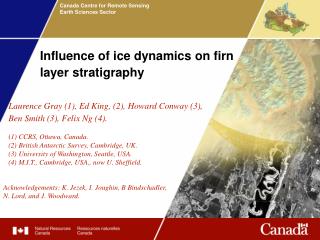
Influence of ice dynamics on firn layer stratigraphy. Laurence Gray (1), Ed King, (2), Howard Conway (3), Ben Smith (3), Felix Ng (4). ( 1) CCRS, Ottawa, Canada. (2) British Antarctic Survey, Cambridge, UK. (3) University of Washington, Seattle, USA.

E N D
Influence of ice dynamics on firn layer stratigraphy Laurence Gray (1), Ed King, (2), Howard Conway (3), Ben Smith (3), Felix Ng (4). (1) CCRS, Ottawa, Canada. (2) British Antarctic Survey, Cambridge, UK. (3) University of Washington, Seattle, USA. (4) M.I.T., Cambridge, USA., now U. Sheffield. Acknowledgements: K. Jezek, I. Joughin, B Bindschadler, N. Lord, and J. Woodward.
Surface radar profiles along the 3 lines show that there is a strong correlation between the RADARSAT ‘flowstripe’ radiometry and the near surface stratigraphy. Relative radiometry km Velocities courtesy Ian Joughin
Another example of the strong correlation between near surface radar stratigraphy and the backscatter magnitude. Depth to the 1951 layer estimated by Ben Smith. Dynamics of the near surface layers and accumulation measurements
Flow stripes correspond to “folds” in the near surface stratigraphy… but how are the folds created and maintained? • ‘Bed bumps’ • Fold creation implies surface topography (slope) variation which could influence the accumulation creating and maintaining the folded layering. • As the stripes appear particularly with lateral compression, often with shear, the forces acting on the firn could directly reinforce and amplify the sub-surface folding. The firn layers are essentially ‘wrinkling’. • Some combination of these mechanisms is possible.
Can ‘isochrones’ be modelled ? … easiest in the along-flow direction… (BAS data from Rutford IS) Ice motion ~ 65 m/a ~105 m/a 5 km
Ice motion ITASE 01-6 39.5 cm/a w.e ITASE 01-5 38.8 cm/a w.e. Kaspari, et al., “Climate variability in West Antarctica derived from annual accumulation rate records from ITASE firn/ice cores”, Ann Glaciol. V39
Implications… • If the model agrees with the GPR data (implying that both the velocity and average accumulation have been constant with historical time) then the average accumulation can be estimated. Using the GPR delay times, the model suggests that the average accumulation (both spatially and temporally) in this area is ~ 0.4-0.5 m. water equivalent per year. This needs to be redone and confirmed ! • We can check for historical velocity change, assuming smaller changes in accumulation.
Some results from the Bindschadler Ice Stream L10 L1 Velocities courtesy Ian Joughin
GPR data and results from BAS Line 1 ~ 45 m/a ~ 22 m/a
Results for BAS Line 10… Not the same as Line 1 ! L10 ~ 60 m/a 5 km ~ 115 m/a 50 100 200 300 400
Summary and Conclusions It is possible to model the way in which GPR layers will evolve with historical time for ice in ‘tributary’ or creep flow. The model works in the flow direction and requires only velocity data and relative accumulation derived from near surface GPR layers. While this work is just beginning, we hope that this capability can be used to … 1). Help provide an estimation of average accumulation (in ‘stable’ areas). 2). If GPR data can be collected especially up-flow from an near-surface core site then it will be easier to resolve whether parts of the core represent changing historical accumulation or the influence of advection of variable up-flow surface accumulation into the core. 3). It may be possible to see historical change in flow.
Model to predict firn layers in the along-flow direction • Assume that… • Over small distances the downstream velocity variation can be written as V = Vo + kx, where k is the longitudinal strain rate , and x is the position along the flow direction. • The transverse strain rate is zero; a 1 m distance across-flow stays as 1 m. So the simulation is 2-dimensional; along-flow and vertical. • With an initial velocity Vo, after time t years a point in the firn will have traveled a distance x = (Vo/k)(exp(kt)-1). • After t years, an along-flow distance of 1m becomes d=exp(kt) • With conservation of material the layer thickness is then = exp(-kt). • The density-depth relation is from Herron and Langway (J. Glaciol. vol 25, 1980), and the permittivity-density relation from Kovacs, Gow and Morey, Cold Reg. Sci. Technol., vol. 23, 1995.