LSA 352 Speech Recognition and Synthesis
1.04k likes | 1.41k Vues
LSA 352 Speech Recognition and Synthesis. Dan Jurafsky. Lecture 6: Feature Extraction and Acoustic Modeling.

LSA 352 Speech Recognition and Synthesis
E N D
Presentation Transcript
LSA 352Speech Recognition and Synthesis Dan Jurafsky Lecture 6: Feature Extraction and Acoustic Modeling IP Notice: Various slides were derived from Andrew Ng’s CS 229 notes, as well as lecture notes from Chen, Picheny et al, Yun-Hsuan Sung, and Bryan Pellom. I’ll try to give correct credit on each slide, but I’ll prob miss some.
Outline for Today • Feature Extraction (MFCCs) • The Acoustic Model: Gaussian Mixture Models (GMMs) • Evaluation (Word Error Rate) • How this fits into the ASR component of course • July 6: Language Modeling • July 19: HMMs, Forward, Viterbi, • July 23: Feature Extraction, MFCCs, Gaussian Acoustic modeling, and hopefully Evaluation • July 26: Spillover, Baum-Welch (EM) training
Outline for Today • Feature Extraction • Mel-Frequency Cepstral Coefficients • Acoustic Model • Increasingly sophisticated models • Acoustic Likelihood for each state: • Gaussians • Multivariate Gaussians • Mixtures of Multivariate Gaussians • Where a state is progressively: • CI Subphone (3ish per phone) • CD phone (=triphones) • State-tying of CD phone • Evaluation • Word Error Rate
Discrete Representation of Signal • Represent continuous signal into discrete form. Thanks to Bryan Pellom for this slide
Digitizing the signal (A-D) • Sampling: • measuring amplitude of signal at time t • 16,000 Hz (samples/sec) Microphone (“Wideband”): • 8,000 Hz (samples/sec) Telephone • Why? • Need at least 2 samples per cycle • max measurable frequency is half sampling rate • Human speech < 10,000 Hz, so need max 20K • Telephone filtered at 4K, so 8K is enough
Digitizing Speech (II) • Quantization • Representing real value of each amplitude as integer • 8-bit (-128 to 127) or 16-bit (-32768 to 32767) • Formats: • 16 bit PCM • 8 bit mu-law; log compression • LSB (Intel) vs. MSB (Sun, Apple) • Headers: • Raw (no header) • Microsoft wav • Sun .au 40 byte header
Discrete Representation of Signal • Byte swapping • Little-endian vs. Big-endian • Some audio formats have headers • Headers contain meta-information such as sampling rates, recording condition • Raw file refers to 'no header' • Example: Microsoft wav, Nist sphere • Nice sound manipulation tool: sox. • change sampling rate • convert speech formats
MFCC • Mel-Frequency Cepstral Coefficient (MFCC) • Most widely used spectral representation in ASR
Pre-Emphasis • Pre-emphasis: boosting the energy in the high frequencies • Q: Why do this? • A: The spectrum for voiced segments has more energy at lower frequencies than higher frequencies. • This is called spectral tilt • Spectral tilt is caused by the nature of the glottal pulse • Boosting high-frequency energy gives more info to Acoustic Model • Improves phone recognition performance
Example of pre-emphasis • Before and after pre-emphasis • Spectral slice from the vowel [aa]
Windowing Slide from Bryan Pellom
Windowing • Why divide speech signal into successive overlapping frames? • Speech is not a stationary signal; we want information about a small enough region that the spectral information is a useful cue. • Frames • Frame size: typically, 10-25ms • Frame shift: the length of time between successive frames, typically, 5-10ms
Common window shapes • Rectangular window: • Hamming window
Discrete Fourier Transform • Input: • Windowed signal x[n]…x[m] • Output: • For each of N discrete frequency bands • A complex number X[k] representing magnidue and phase of that frequency component in the original signal • Discrete Fourier Transform (DFT) • Standard algorithm for computing DFT: • Fast Fourier Transform (FFT) with complexity N*log(N) • In general, choose N=512 or 1024
Discrete Fourier Transform computing a spectrum • A 24 ms Hamming-windowed signal • And its spectrum as computed by DFT (plus other smoothing)
Mel-scale • Human hearing is not equally sensitive to all frequency bands • Less sensitive at higher frequencies, roughly > 1000 Hz • I.e. human perception of frequency is non-linear:
Mel-scale • A mel is a unit of pitch • Definition: • Pairs of sounds perceptually equidistant in pitch • Are separated by an equal number of mels: • Mel-scale is approximately linear below 1 kHz and logarithmic above 1 kHz • Definition:
Mel Filter Bank Processing • Mel Filter bank • Uniformly spaced before 1 kHz • logarithmic scale after 1 kHz
Mel-filter Bank Processing • Apply the bank of filters according Mel scale to the spectrum • Each filter output is the sum of its filtered spectral components
Log energy computation • Compute the logarithm of the square magnitude of the output of Mel-filter bank
Log energy computation • Why log energy? • Logarithm compresses dynamic range of values • Human response to signal level is logarithmic • humans less sensitive to slight differences in amplitude at high amplitudes than low amplitudes • Makes frequency estimates less sensitive to slight variations in input (power variation due to speaker’s mouth moving closer to mike) • Phase information not helpful in speech
The Cepstrum • One way to think about this • Separating the source and filter • Speech waveform is created by • A glottal source waveform • Passes through a vocal tract which because of its shape has a particular filtering characteristic • Articulatory facts: • The vocal cord vibrations create harmonics • The mouth is an amplifier • Depending on shape of oral cavity, some harmonics are amplified more than others
Vocal Fold Vibration UCLA Phonetics Lab Demo
We care about the filter not the source • Most characteristics of the source • F0 • Details of glottal pulse • Don’t matter for phone detection • What we care about is the filter • The exact position of the articulators in the oral tract • So we want a way to separate these • And use only the filter function
The Cepstrum • The spectrum of the log of the spectrum Spectrum Log spectrum Spectrum of log spectrum
Mel Frequency cepstrum • The cepstrum requires Fourier analysis • But we’re going from frequency space back to time • So we actually apply inverse DFT • Details for signal processing gurus: Since the log power spectrum is real and symmetric, inverse DFT reduces to a Discrete Cosine Transform (DCT)
Another advantage of the Cepstrum • DCT produces highly uncorrelated features • We’ll see when we get to acoustic modeling that these will be much easier to model than the spectrum • Simply modelled by linear combinations of Gaussian density functions with diagonal covariance matrices • In general we’ll just use the first 12 cepstral coefficients (we don’t want the later ones which have e.g. the F0 spike)
Dynamic Cepstral Coefficient • The cepstral coefficients do not capture energy • So we add an energy feature • Also, we know that speech signal is not constant (slope of formants, change from stop burst to release). • So we want to add the changes in features (the slopes). • We call these delta features • We also add double-delta acceleration features
Delta and double-delta • Derivative: in order to obtain temporal information
Typical MFCC features • Window size: 25ms • Window shift: 10ms • Pre-emphasis coefficient: 0.97 • MFCC: • 12 MFCC (mel frequency cepstral coefficients) • 1 energy feature • 12 delta MFCC features • 12 double-delta MFCC features • 1 delta energy feature • 1 double-delta energy feature • Total 39-dimensional features
Why is MFCC so popular? • Efficient to compute • Incorporates a perceptual Mel frequency scale • Separates the source and filter • IDFT(DCT) decorrelates the features • Improves diagonal assumption in HMM modeling • Alternative • PLP
Problem: how to apply HMM model to continuous observations? • We have assumed that the output alphabet V has a finite number of symbols • But spectral feature vectors are real-valued! • How to deal with real-valued features? • Decoding: Given ot, how to compute P(ot|q) • Learning: How to modify EM to deal with real-valued features
Vector Quantization • Create a training set of feature vectors • Cluster them into a small number of classes • Represent each class by a discrete symbol • For each class vk, we can compute the probability that it is generated by a given HMM state using Baum-Welch as above
VQ • We’ll define a • Codebook, which lists for each symbol • A prototype vector, or codeword • If we had 256 classes (‘8-bit VQ’), • A codebook with 256 prototype vectors • Given an incoming feature vector, we compare it to each of the 256 prototype vectors • We pick whichever one is closest (by some ‘distance metric’) • And replace the input vector by the index of this prototype vector
VQ requirements • A distance metric or distortion metric • Specifies how similar two vectors are • Used: • to build clusters • To find prototype vector for cluster • And to compare incoming vector to prototypes • A clustering algorithm • K-means, etc.
Distance metrics • Simplest: • (square of) Euclidean distance • Also called ‘sum-squared error’
Distance metrics • More sophisticated: • (square of) Mahalanobis distance • Assume that each dimension of feature vector has variance 2 • Equation above assumes diagonal covariance matrix; more on this later
Training a VQ system (generating codebook): K-means clustering 1. Initialization choose M vectors from L training vectors (typically M=2B) as initial code words… random or max. distance. 2. Search: for each training vector, find the closest code word, assign this training vector to that cell 3. Centroid Update: for each cell, compute centroid of that cell. The new code word is the centroid. 4. Repeat (2)-(3) until average distance falls below threshold (or no change) Slide from John-Paul Hosum, OHSU/OGI