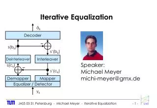
Iterative Equalization
Iterative Equalization. â k. Decoder. s(b k ). s‘(b k ). Deinterleaver. Interleaver. Speaker: Michael Meyer michi-meyer@gmx.de. s(c k ). s‘(c k ). Demapper. Mapper. Equalizer / Detector. y k. System Configuration and Receiver Structures. a k. â k. â k. â k. Encoder. Decoder.

Iterative Equalization
E N D
Presentation Transcript
Iterative Equalization âk Decoder s(bk) s‘(bk) Deinterleaver Interleaver Speaker: Michael Meyer michi-meyer@gmx.de s(ck) s‘(ck) Demapper Mapper Equalizer / Detector yk
System Configuration and Receiver Structures ak âk âk âk Encoder Decoder Decoder bk s(bk) s(bk) Interleaver Deinterleaver s‘(bk) Deinterleaver Interleaver ck s(ck) s(ck) Mapper Demapper s‘(ck) xk s(xk) Optimal Detector Demapper Mapper Channel Equalizer / Detector Equalizer / Detector yk yk yk yk System Configuration Receiver A: optimal detector Receiver B: one-time equalization and detection Receiver C: turbo equalization
Interleaver ak Encoder bk Interleaver ck Mapper xk Example for an interleaver: A 3-random interleaver for 18 code bits Channel yk
Equalization • Methods to compensate the channel effects Transmitter Receiver e.g. Multi-Path Propagation might lead to Intersignal Interference (ISI).
Used Channel Modell t t In the following, we will use an AWGN channel with known channel impulse response (CIR). The received signal is given by channel coefficient sent signal noise In matrix form: y = Hx + n As an example, we have a length-three channel with h0=0.407 h1=0.815 h2=0.407 The noise is Gaussian:
The Forward / Backward Algorithm • For Receiver B, the Forward / Backward Algorithm is often used for equalization and decoding. • As this algorithm is a basic building block for our turbo equilization setup, we will discuss it in detail • for equalization • for decoding • We will continue our example to make things clear. • The example uses binary phase shift keying (BPSK)
The Decision Rule The decision rule for the equalizer is âk Decoder Deinterleaver with the log-likelihood ratio Demapper s(xk) Equalizer / Detector yk So, we have to calculate L(c|y) Receiver B:
The Trellis Diagram (1) (-1, -1) (-1, -1) (1, -1) (1, -1) (-1, 1) (-1, 1) (1, 1) (1, 1) state rj state ri inputxk=xi,j output vk=vi,j time k+2 A branch of the trellis is a four-tuple (i, j, xi,j, vi,j)
The Trellis Diagram (2) t t 2L = 4 If the tapped delay line contains L elements and if we use a binary alphabet {+1, -1}, the channel can be in one of 2L states ri. The set of possible states is S = {r0,r1,…,r2L-1} At each time instance k=1,2,…,N the state of the channel is a random variable sk S.
The Trellis Diagram (3) Using a binary alphabet, a given state sk = ri can only develop into two different states sk+1 = rj depending on the input symbol xk = xi,j = {+1, -1}. The output symbol vk = vi,j in the noise-free case is easily calculated by v2,0 = h0x2,0 + h1x3,2 + h2x3,3 = 0.407∙1 + 0.815∙1 + 0.407∙(-1) = 0.815
The Trellis Diagram (4) xi,j and vi,j are uniquely identified by the index pair (i j). The set of all index pairs (i j) corresponding to valid branches is denoted B. e.g B = {(00), (01), (12), (13), (20), (21), (33), (32)}
The Joint Distribution p(sk, sk+1, y) As we are separating the equalization from the decoding task, we assume that the random variables xk are statistically independent (IID), hence We then have to calculate P(sk=ri, sk+1=rj | y). This is the probability that the transmitted sequence path in the trellis contains the branch (I, j, xi,j, vi,j) at the time instance k. This APP (a posteriori probability) can be computed efficiently with the forward / backward algorithm, based on a suitable decomposition of the joint distribution p(sk, sk+1, y) = p(y) ∙ P(sk, sk+1 | y)
The Decomposition We can write the joint distribution as p(sk, sk+1, y) = p(sk, sk+1, (y1,…,yk-1), yk, (yk+1,…,yN)) and decompose it to probability that contains all paths through the Trellis to come to state sk probability for the transition from sk to sk+1 with symbol yk probability that contains all possible pathes from state sk+1 to sN yk … … so s1 sk sk+1 sN-1 sN
The Transition Probability γ We can further decompose the transition probability into k(sk, sk+1) = P(sk+1|sk) ∙ p(yk|sk, sk+1) Using the index pair (i j) and the set B we get From the channel law yk=vk+nk and the Gaussian distribution we know that k(r0, r3) = 0 as (03) B k(r0, r0) = P(xk=+1)∙p(yk|vk=1.63)
The Probability (Forward) The term k(s) can be computed via the recursion with the initial value 0(s) = P(s0=s). 2(s2) 1(s1) 1(s1,s2) ri rj … so s1 s2 Note: k contains all possible paths leading to sk.
The Probability β (Backward) Analogous, the term βk(s) can be computed via the recursion with the initial value βN(s) = 1 for all s S. β2(s2) 2(s2,s3) β3(s3) ri rj yk … … s2 s3 sN
The Formula For The LLR Now, we know the APP P(xk = x|y). All we need to accomplish this task is to sum the branch APPs P(sk, sk+1|y) over all branches that correspond to an input symbol xk=x To compute the APP P(xk=+1|y) the branch APPs of the index pairs (00),(12),(20) and (32) have to be summed over -1
The FBA in Matrix Form For convenience, the forward/backward algorithm may also be expressed in matrix-form. We need to create two matrices. Pk |S|x|S| with {Pk}I,j = k(ri, rj) A(x) |S|x|S| with A third matrix is created by elementwise multiplication: B(x) = A(x)∙Pk |S|x|S|
The Algorithm Input: Matrices Pk and Bk(x) We calculate vectors fk |S|x1 and bk |S|x1 Initialize with f0 = 1 and bN = 1 For k = 1 to N step 1 (forward) fk = Pk-1fk-1 For k = N to 1 step -1 (backward) bk=PkTbk+1 Output the LLRs:
Soft Processing âk Decoder A natural choice for the soft information s(xk) are the APPs or similarly the LLRs L(ck|y), which are a “side product” of the maximum a-posteriori probability (MAP) symbol detector. Also, the Viterbi equalizer may produce approximations of L(ck|y). For filter-based equalizers extracting s(xk) is more difficult. A common approach is to assume that the estimation error is Gaussian distributed with PDF p(ek)… s(bk) Deinterleaver s(ck) Demapper s(xk) Equalizer / Detector yk
Decoding - Basics • Convert the LLR L(ck|y) back to probabilities: • Deinterleave P(ck|y) to P(bk|y) • is the input set of probabilities to the decoder • With the forward/backward algorithm we may again calculate the LLR L(ak|p) For the example: Encoder of a convolutional code, where each incoming data bit ak yields two code bits (b2k-1, b2k) via b2k-1 = ak ak-2 b2k = ak ak-1 ak-2 t t
Decoding - Trellis (1,1) (1,1) (0,1) (0,1) (1,0) (1,0) (0,0) (0,0) state rj state ri inputak=ai,j output (b2k-1, b2k)=(b1,i,j, b2,i,j) The convolutional code yields to a new trellis with branches denoted by the tuple (i, j, ai,j, b1,i,j, b2,i,j). Set B remains {(00),(01),(12),(13),(20),(21),(33),(32)}
Decoding – Formulas (1) To apply the forward/backward algorithm, we have to adjust the way Pk and A(x) are formed. For Pkwe have to redefine the transition probability . {Pk}I,j = k(ri, rj) Ba(x) = Aa(x)∙Pk
Decoding – Formulas (2) So, we calculate L(ak|p) using the forward / backward algorithm. By changing A(x) we can also calculate L(b2k-1|p) and L(b2k|p) which will later serve as a priori information for the equalizer. L(b2k-1|p): L(b2k|p): with the set of probabilities:
Decoding - Example L(ak|p): L(b2k-1|p): L(b2k|p):
Decoding - Algorithm For decoding, we may use the same forward/backward algorithm with different initialization, as the encoder has to terminate at the zero state at time steps k=0, k=K. Change Bk(x) to output L(b2k-1|p) or L(b2k|p). Input: Matrices Pk and Bk(x) Initialize with f0 = [1 0…0]T |S|x1 and bN = [1 0…0]T |S|x1 For k = 1 to N step 1 (forward) fk = Pk-1fk-1 For k = N to 1 step -1 (backward) bk=PkTbk+1 Output the LLRs:
Bit Error Rate (BER) With soft information, we may gain 2dB, but it is still a long way to -1.6 dB. Performance of separate equalization and decoding with hard estimates (dashed lines) or soft information (solid lines). The System transmits K=512 data bits and uses a 16-random interleaver to scramble N=1024 code bits.
Block Diagram - Separated Concept Observations a Posteriori Probabilities Forward/ Backward Algorithm Observations a Posteriori Probabilities Equalizer Forward/ Backward Algorithm Prior Probabilities y Prior Probabilities L(ck|y) Block diagram of the f/b algorithm Let’s look again at the transition propability: . Deinterleaver local evidence about which branch in the trellis was transversed. Prior information L(bk|y) L(bk|p) • So far: • The equalizer does not have any prior knowledge available, so the formation of entries in Pk relies solely on the observation y. • The decoder forms the corresponding entries in Pk without any local observations but entirely based on bitwise probabilities P(bk|y) provided by the equalizer. Decoder Forward/ Backward Algorithm Prior Prob. a Posteriori Probabilities Observations L(ak|p) Decision Rule âk
Block Diagram - Turbo Equalization Observations Observations a Posteriori Probabilities a Posteriori Probabilities Equalizer Forward/ Backward Algorithm Equalizer Forward/ Backward Algorithm y y Turbo Equalization Prior Probabilities Prior Probabilities L(ck|y) L(ck|y) Lext(ck|p) _ + Let’s look again at the transition propability: Extrinsic Information Lext(ck|y) . Interleaver Extrinsic Information Lext(bk|p) Deinterleaver Deinterleaver local evidence about which branch in the trellis was transversed Prior information _ + Lext(bk|y) L(bk|p) L(bk|p) • So far: • The equalizer does not have any prior knowledge available, so the formation of entries in Pk relies solely on the observation y • The decoder forms the corresponding entries in Pk without any local oobservations but entirely based on bitwise probabilities P(bk|y) provided by the equalizer. Decoder Forward/ Backward Algorithm Decoder Forward/ Backward Algorithm Prior Prob. Prior Prob. a Posteriori Probabilities a Posteriori Probabilities Observations Observations L(ak|p) L(ak|p) Decision Rule Decision Rule âk âk
Block Diagram - Comparison Observations Observations Observations a Posteriori Probabilities a Posteriori Probabilities a Posteriori Probabilities Equalizer Forward/ Backward Algorithm Equalizer Forward/ Backward Algorithm Equalizer Forward/ Backward Algorithm y y y Prior Probabilities Prior Probabilities Prior Probabilities L(ck|y) L(ck|y) L(ck|y) Lext(ck|p) _ + Extrinsic Information Lext(ck|y) Interleaver Extrinsic Information Lext(bk|p) Deinterleaver Deinterleaver Deinterleaver _ + Lext(bk|y) L(bk|y) L(bk|p) L(bk|p) L(bk|p) Decoder Forward/ Backward Algorithm Decoder Forward/ Backward Algorithm Decoder Forward/ Backward Algorithm Prior Prob. Prior Prob. Prior Prob. a Posteriori Probabilities a Posteriori Probabilities a Posteriori Probabilities Observations Observations Observations L(ak|p) L(ak|p) L(ak|p) Receiver B: separated equalization and detection Receiver C: Turbo Equalization Decision Rule Decision Rule Decision Rule âk âk âk
Turbo Equalization - Calculation Observations Observations a Posteriori Probabilities a Posteriori Probabilities Equalizer Forward/ Backward Algorithm Equalizer Forward/ Backward Algorithm Caution: We have to split L(ck|y)=Lext(ck|y) + L(ck) as only extrinsic information is fed back. Lext(ck|y) does not depend on L(ck). L(ck) would create direct positive feedback converging usually far from the globally optimal solution. The interleavers are included into the iterative update loop to further disperse the direct feedback effect. The forward/backward algorithm creates locally highly correlated output. These correlations between neighboring symbols are largely suppressed by the interleaver. y y Prior Probabilities Prior Probabilities L(ck|y) L(ck|y) Lext(ck|p) _ + Extrinsic Information Lext(ck|y) Interleaver Extrinsic Information Lext(bk|p) Deinterleaver Deinterleaver _ + Lext(bk|y) L(bk|p) L(bk|p) Decoder Forward/ Backward Algorithm Decoder Forward/ Backward Algorithm Prior Prob. Prior Prob. a Posteriori Probabilities a Posteriori Probabilities Observations Observations L(ak|p) L(ak|p) Decision Rule Decision Rule âk âk
Turbo Equalization - Algorithm Input: Observation sequence y Channel coefficients hl for l=0,1,…,L Initialize: Predetermine the number of iterations T Initialize the sequence of LLRs Lext(c|p) to 0 Compute recursively for T iterations L(c|y) = Forward/Backward(Lext(c|p)) Lext(c|y) = L(c|y) – Lext(c|p) L(b|p) = Forward/Backward(Lext(b|y)) Lext(b|p) = L(b|p) – Lext(b|y) Output: Compute data bit estimates âk from L(ak|y)
Turbo Equalization - BER The system transmits K=512 data bits and uses a 16-random interleaver to scramble N=1024 code bits. Figure A uses separate equalization and detection. Figure B uses turbo MMSE Equalization with 0, 1, 2, 10 iterations. Figure C uses turbo MAP equalization after the same iterations. The line marked with “x” is the performance with K = 25000 and 40-random interleaving after 20 iterations. A B C Turbo MMSE Turbo MAP
Turbo Equalization – Exit Charts [2] Receiver EXIT chart at 4 dB ES/N0 Receiver EXIT chart at 0.8 dB ES/N0
Linear Equalization • The computational effort is so far determined by the number of trellis states. An 8-ary alphabet gives 8L states in the trellis. • Linear filter-based approaches perform only simple operations on the received symbols, which are usually applied sequentially to a subset of M observed symbols yk. e.g. yk=(yk-5 yk-4 … yk+5)T M=11 A channel of length L can be expressed as with M x (M+L). Any type of linear processing of yk to compute can be expressed as . The channel law immediately suggests , the zero-forcing approach. With noise present, an estimate is obtained. This approach suffers from “noise enhancement”, which can be severe if is ill conditioned. This effect can be avoided using linear minimum mean square error (MMSE) estimation minimizing . The equation used is It is also possible to nonlinearly process previous estimates to find the besides the linear processing of yk (decision-feedback equalization (DFE).
Complexity [2] M: Channel impulse response length N: Equalizer filter length 2m: Alphabet length of the signal constellation DFE: Decision Feedback Equalization
Comparison • The MMSE approaches have reduced complexity. • The MMSE approaches perform as well as the BER-optimal MAP approach, only requiring a few more iterations. • However, the MAP equalizer may handle SNR ranges where all other approaches fail. Ideas • treat scenarios with unknown channel characteristics, e. g. combined channel estimation and equalization using a-priori information • Switch between MAP and MMSE algorithms depending on fed back soft information
Thank you for your attention! Questions & Comments ?
References [1] Koetter, R.; Singer, A.; Tüchler, M.: Turbo Equalization IEEE Signal Processing Magazine, vol. 21, no. 1, pp 67-80, Jan 2004 [2] Tüchler, M.; Koetter, R.; Singer, A.: Turbo Equalization: Principles and New Results IEEE Trans. Commun., vol. 50, pp. 754-767, May 2002 [3] Tüchler, M.; Singer, A.; Koetter, R.: Minimum Mean Squared Error Equalization Using A-priori Information IEEE Trans. Signal Processing, vol. 50, pp. 673-683, March 2002