Using the Instrumental Variables Technique in Educational Research
430 likes | 1.29k Vues
Using the Instrumental Variables Technique in Educational Research. By Larry V. Hedges Northwestern University. Outline. The place of IV in educational research methodology The classical econometric justification of IV The modern statistical approach to IV and causal inference

Using the Instrumental Variables Technique in Educational Research
E N D
Presentation Transcript
Using the Instrumental Variables Technique in Educational Research By Larry V. Hedges Northwestern University
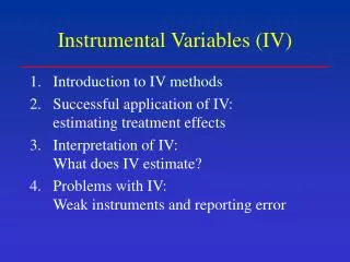
Outline • The place of IV in educational research methodology • The classical econometric justification of IV • The modern statistical approach to IV and causal inference • Implementing IV analyses • What can go wrong • Practical problems in IV
Disclaimer This talk is intended to be non-technical, therefore: No matrix algebra will be used Some technical details will be glossed over For example, I will speak of bias and accuracy in situations where the actual moments of estimates do not exist The object is to build intuition and understanding not to be rigorously technically correct
Estimating Treatment Effects Consider treatment assignment (dummy variable) X and outcome Y Regress Y on X Yi = β0 + β1Xi + εi The estimate of β1 is just the difference between the mean Y for X = 1 (the treatment group) and the mean Y for X = 0 (the control group) Thus the OLS estimate is = β1 +
Estimating Treatment Effects(With Random Assignment) If the treatment is randomly assigned, then X is uncorrelated with ε(X is exogenous) If X is uncorrelated with εif and only if But if , then the mean difference is = β1 + = β1 This implies that standard methods (OLS) give an unbiased estimate of β1, which is the average treatment effect That is, the treatment-control mean difference is an unbiased estimate of β1,
What goes wrong without randomization?(Simple Case) If we do not have randomization, there is no guarantee that X is uncorrelated with ε(X may be endogenous) Thus the OLS estimate is still = β1 + If X is correlated with ε, then Hence does not estimate β1, but some other quantity that depends on the correlation of X and ε If X is correlated with ε, then standard methods give a biased estimate of β1
What goes wrong without randomization? When you regress Y on X, Y = β0 + β1X + ε and the OLS estimate of β1 can be described as But since X and εare correlated, bOLS does not estimateβ1 but some other quantity that depends on the correlation of X and ε
Instrumental Variables Natural experiments are naturally occurring situations where we want to know the effect of variable X on Y and there is a variable Z related to X, but not ε Another way so say this is: Z effects Y only through X This variable Z is called an instrumental variable It can be shown that is an unbiased estimator of β1in large samples but not in small samples (bIV is consistent)
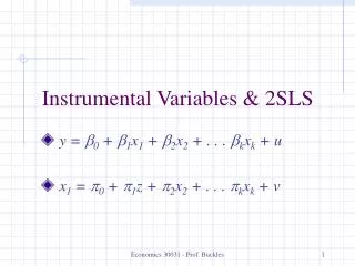
Instrumental Variables One way to see this is in terms of two regression equations Yi = β0 + β1Xi + εi Xi = γ0 + γ1Zi + ηi Note that, in this model X is endogenous (may be correlated with ε) The instrumental variables model requires that: 1. γ1 ≠ 0 so that Z predicts X, and 2. Z uncorrelated with ε (Z is exogenous) [Cov{ε, Z} = 0]
Instrumental Variables You can see the logic of IV as follows
Instrumental Variables Recall the two regression equations Yi = β0 + Xiβ1 + εi Xi = γ0 + Ziγ1 + ηi This is why instrumental variables methods are associated with simultaneous equations methods in econometrics In this formulation, Zi and Xi can be vectors, so you can have • several X variables, only some of which are endogenous and • several Z variables only some of which are instruments (but you must have more instruments than endogenous X variables) The instrumental variables model requires that γ1 ≠ 0 and Z uncorrelated with ε
Instrumental Variables Remember: To be an instrument Z must be: • Relevant (Z must be related to the endogenous variable X) • Exogenous (Z must be related to the outcome Yonly through X) Failure of either condition is a problem! But both conditions can be hard to satisfy at the same time
ExampleExperiments with imperfect compliance Effect of intent to treat, versus treatment on the treated Intent to treat estimate Compare Y for all those assigned to treatment 1 to those assigned to treatment 0 This estimates the causal effect on Y of assignment to treatment It does not measure the effect of actually receiving the treatment unless there is perfect compliance Experimental methods cannot estimate the effect of receiving the treatment, because that cannot be randomly assigned (without perfect compliance) For example, families that use vouchers may be systematically different than those who do not in ways that affect Y
ExampleExperiments with imperfect compliance Voucher experiments We may want to know the causal effect of using vouchers But not all families assigned vouchers use them Because use of vouchers is not randomly assigned, it may be correlated with residuals Random assignment to receive vouchers (is?) an instrument because • Voucher assignment is related to voucher use • Voucher assignment may affect school achievement only through voucher use
ExampleExperiments with imperfect compliance This same idea can be applied to study the effect of receiving treatment (the effect of treatment on the treated) in many settings It can also be used to study the effect of the “active ingredients” in imperfectly implemented treatments It can (more cautiously) be used to study effects of a treatment where there is an instrument that does not arise via random assignment
Estimating Causal Effects The Rubin-Holland-Rosenbaum model starts with 2 potential responses for each unit r1i = outcome unit i experiences in treatment 1 r0i = outcome unit i experiences in treatment 0 The causal effect of treatment 1 versus 0 on unit i is defined as τi = r1i – r0i You can’t estimate τi directly, but you can estimate the average causal effect in some circumstances, like a randomized experiment
Estimating Causal Effects (Randomized Experiments) Let Z = {0, 1} be a variable that expresses treatment assignment In a perfectly implemented randomized experiment, treatment assignment (Z) is uncorrelated with both r1i and r0i, so E{r1i | treatment 1 (Z = 1)} = E{r1i} E{r0i | treatment 0 (Z = 0)} = E{r0i} Thus E{r1 | Z = 1} – E{r0 | Z = 0} = E{r1 – r0} = So the estimate of the treatment effect is unbiased
Estimating Causal Effects (IV Studies) Consider IV within randomized experiments Random assignment Z, with endogenous X (believed to be the efficacious causal component of treatment) We want to know the causal effect of the endogenous variable X on outcome Y For example • Effect of voucher use in randomized choice studies • Effect of treatment implementation • Effect of using specific instructional methods
Estimating Causal Effects (IV Studies) IV can estimate causal effects of X on Y, if the following assumptions hold: • SUTVA • Random assignment of Z • Exclusion restriction (exogeneity of Z) • Nonzero causal effect of Z on X • Monotonicity (no defiers) Then the IV estimate is an estimate of the average treatment effect for those who comply with assignment
Unit’s Reaction to Treatment We can characterize unit’s reaction to treatment into four categories • Compliers (do what they are assigned to do) • Always takers (get treatment regardless of assignment) • Never takers (never get treatment regardless of assignment) • Defiers (always do the opposite of what is assigned) [Note that we ruled out defiers by hypothesis] Note that we cannot necessarily identify individuals are which
Estimating Causal Effects (IV Studies) Note that the causal effect of treatment on always takers and never takers is 0 by definition We can also see the IV estimate as the ratio of two causal effects (two intent to treat estimates)
Carrying Out IV Analyses Recall the description of IV in terms of two regression equations Yi = β0 + β1Xi + εi Xi = γ0 + γ1Zi + ηi Two-stage least squares estimation involves • Regressing X on Z to get estimates of X • Regressing Y on to get an estimate of β1 Specialized programs are also available in many packages (e.g., STATA or SAS) There are also other, more complex procedures (such as LIML)
What Can Go Wrong In the Use of IV Failure of the assumptions! Failure of exogeneity (Z influences Y though other variables than X) Failure of relevance (Z has only a weak relation to X) Both of these kinds of failures are quantitative, not qualitative Choice of instruments may involve a tradeoff between these two kinds of failures But also, IV is a large sample procedure, even when assumptions are met it is only guaranteed to be unbiased in large samples
Violation of IV Assumptions It is important to distinguish between two situations: 1. The assumption of exogeneity is met exactly and the relevance may be small (but nonzero) [weak instruments] In this case the only bias is due to small sample bias in estimation 2. The exogeneity assumption is not met exactly In this case there is additional (large sample) bias due to direct causal effect of Z on Y The analysis of bias is quite different in these two cases!
Exogenous, but Weak Instruments Even when assumptions are perfectly met, IV is not unbiased in small (finite) samples Finite sample bias can be non-negligible (e.g., 20 - 30%), even when the sample size is over 100,000 if the instrument is weak (Z is only weakly correlated with X) The relative bias of bIV (versus bOLS) is approximately 1/F where F is the F-statistic for testing the relation between the instrument (Z) and endogenous variable (X) A small value of F, even if it is large enough to be statistically significant signals possible large bias in bIV
Exogenous, but Weak Instruments Measuring strength of instruments: The concentration parameter One interpretation of the concentration parameter is related to the F-test statistic in the regression of X on Z is a test of the hypothesis that γ = 0: k(F – 1) estimates λ where k is the number of instruments The accuracy of bIV (2SLS) estimate depends on λ, (λfunctions like a sample size)
Testing for Weak Instruments It is not sufficient that the relation between Z and X is statistically significant Need to test whether λ/k exceeds a threshold (below which instruments are weak enough to imperil inference) Two definitions of ‘weak enough to imperil inference,’ and both can be tested with first stage F for relation of Z and X(Stock & Yugo, 2005): 1. Bias of bIV exceeds 10% of the bias of bOLS Requires F > 10 2. Actual level of 5% significance test exceeds 15% Requires F > 24
Exogenous, but Weak Instruments Exact (small sample) results are available, but very complex (almost to the point of being uninformative) In general, more instruments increases the relevance of the instrument set (increases the first stage F) But, too many instruments increases small sample bias (compared to few instruments) In general it is best to have as few instruments as possible, and for them to be strongly correlated with X (the endogenous variable)
There are Several IV Methods I focused on 2SLS, the most widely used IV method There are more complex competitors, such as the Limited Information Maximum Likelihood (LIML) estimation Analyses of these methods are difficult too. Large sample methods can help, but There are at least 4 different large sample (asymptotic) models for analyzing IV (and they often give different results) One of these suggests that 2SLS is equivalent to LIML Small sample studies (not definitive) suggest that LIML may be superior to 2SLS in small samples
There are Several IV Methods But the full story is not completely clear (e.g., how much this finding depends on normality) and it is not simple Although it is generally found that 2SLS has particularly poor finite sample behavior, each alternative estimator seems to have its own pathologies when instruments are weak. (Andrews & Stock, 2005, p. 2)
Failure of Exogeneity Let H be the direct causal effect of Z on Y Then if the exclusion restriction (exogeneity) is violated, the (large sample, large λ) bias in bIV is This shows that bias is reduced when the instrument is relevant (strong correlation between Z and X), so the odds of being a noncomplier are small
Failure of Exogeneity Failure of exogeneity may introduce large biases that are hard to quantify precisely because they depend on unobservables Usually, this assumption will be (somewhat) false The best we can do is often to be skeptical and to make sure exogeneity is highly plausible in the setting to which we apply IV
IV Can Provide Valid Estimates There are applications in which IV does provide credible estimates Krueger’s (1999) IV estimate of the effects of actual class size on achievement using randomization as an instrument Howell et al.’s (2000) IV estimate of the effects of using school vouchers on achievement using randomization as an instrument Bloom et al.’s (1997) IV estimate of the effects of JTPA on earnings using randomization as an instrument
Practical Problems with IV How do we know if Z is exogenous? Isn’t randomization always a good instrument? No! Consider a randomized experiment to change instruction (using many sites or schools)
Practical Problems with IV Z is assignment to treatment to change instruction X is a measure of the instruction targeted by treatment Is Z relevant (a strong instrument)? Hard to tell a priori (e.g., if Z is dichotomous, X is continuous, Z may not explain much variance in X) Is Z (exogenous)? Why should Znot influence Y through other unmeasured instructional practices?
Practical Problems with IV Possible Solution Include other instructional practices as covariates or endogeneous variables But the number of instruments must exceed the number of endogenous variables—now we need more instruments We could include Z-by-site interactions as instruments But now we have increased the number of instruments, which may increase bias
Practical Problems with IV Assignment may have direct effects on Y if volunteers want the treatment (Shadish, Cook, & Campbell, 2002) Assignment may influence units to get alternatives • Tutoring • Teacher induction • Health care • After school programs Assignment may have a discouraging effect on control group
Conclusions IV can make possible estimates of causal effects without random assignment in some cases But it is no panacea Often, it will be difficult to find instruments that are both relevant (strong enough) and exogenous IV estimation is a complicated subject and good theory for all of the relevant issues is not available For example, all of the theory I have mentioned assumes simple random sampling so it does not take clustered sampling (of the kind in most education experiments) into account
Select Bibliography Causal Inference Rubin, D. B. (1974). Estimating causal effects in randomized and non-randomized studies. Journal of Educational Psychology, 66, 688-701. Angrist, J. D., Imbens, G. W., & Rubin, D. B. (1996). Identification of causal effects using instrumental variables. Journal of the American Statistical Association, 91, 444-455. Imbens, G. W. & Angrist, J. D. (1994). Identification and estimation of local average treatment effects. Econometrica, 62, 467-475. Natural Experiments Angrist, J. D. & Krueger, A. B. (2000). Instrumental variables and the search for identification: From supply an demand to natural experiments. The Journal of Economic Perspectives, 15, 69-85.
Select Bibliography Weak Instruments Bound, J., Jaeger, D. A., & Baker, R. M. (1995). Problems with instrumental variables estimation when the correlation between the instruments and the endogenous explanatory variable is weak, Journal of the American Statistical Association, 90, 443-450. Staiger, D., & Stock, J. H. (1997). Instrumental variables regression with weak instruments. Econometrica, 65, 557-586. Nelson, C. R. & Startz, R. (1990). Some further results on the exact small sample properties of the instrumental variable estimator. Econometrica, 58, 967-976. Stock, J. H., Wright, J. H., & Yogo, M. (2002). A survey of weak instruments and weak identification in generalized method of moments. Journal of Business and Economic Statistics, 20, 518-529 Buse, A. (1992). The bias of instrumental variable estimators. Econometrica, 60, 173-180.