Static or fixed variables
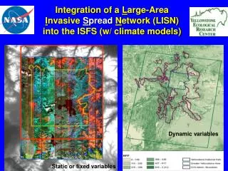
Integration of a L arge-Area I nvasive S pread N etwork (LISN) into the ISFS (w/ climate models). Dynamic variables. Static or fixed variables. General Outline. NASA Invasive Ecological Forecasting (include Jackie’s thesis and other work) Review original GYCC project

Static or fixed variables
E N D
Presentation Transcript
Integration of a Large-Area Invasive SpreadNetwork (LISN) into the ISFS (w/ climate models) Dynamic variables Static or fixed variables
General Outline • NASA Invasive Ecological Forecasting (include Jackie’s thesis and other work) • Review original GYCC project • Details of the NASA project and some initial results from last two summers a. preliminary summary of field data b. preliminary analysis of RS data 4. Approaches to mapping WBP blister rust and mountain pine beetle
Team, Partners/Collaborators • Bob Crabtree, PI, Yellowstone Ecological Research Center • John Schnase, co-I, NASA-Goddard Space Flight Center • Chris Potter, co-I, NASA-Ames Research Center • Paul Moorcroft, co-I, Harvard University • Shengli Huang, co-I, Yellowstone Ecological Research Cntr. • Josh Harmsen, Ph.D. student, U.C.- Berkeley & YERC • Jackie Hatala, Staff Scientist, Harvard University & YERC • Randy Mullen, Ecological Statistician, YERC Collaborators: Mary Maj, GYCC and GYCC Weeds Committee; Jeff Pettingill, Idaho Falls, Nancy Glenn, ISU; Jack Norland, NDSU; Craig McClure, YNP; Rob Mickelsen/Kyle Moore/Bryce Fowler/Walt Grows, Caribou-Targhee National Forest; and Bruce Maxwell/Lisa Rew, MSU; Diana Six, University of Montana; USDA-ARS; David Bubenheim, NASA-ARC; Jeff Morrisette…
NASA LISN OBJECTIVE(S) • Develop Hierarchical Bayesian models for predicting invasive weed (& pathogen) spread over time (Ecological Forecasting program) • Investigate 4 species of biological and economic importance: leafy spurge, Canada thistle, blister rust, and cheatgrass at ecosystem scales • Incorporate dynamic climate data, carbon-climate model output, and 3-D vegetation structure as covariates for future predictions • Add a large regional ecosystem (GYE) with new agency partners to the existing NISFS • Validate, compare, disseminate (publish) and benchmark models and integrate with the NISFS
Hyperspectral Data Analysis of Whitebark Pine (Pinus albicaulis) and White Pine Blister Rust (Cronartium ribicola) at 4 Sites in the GYE • Don Despain, BRD, U.S. Geological Survey • Chuck Schwartz, Leader, Interagency Grizzly Bear • Study Team, Bozeman, MT • Ward McCaughey, Director, USFS Northern Rockies • Experiment Station, Bozeman, MT • Kerry Halligan, Yellowstone Ecological Research Center • Bob Crabtree, Yellowstone Ecological Research Center Collaborators: Roy Bergstrom, Shoshone National Forest Dan Reinhart, Yellowstone National Park Field and Research Assistants: Sarah Elmendorf, Justin Pidot, Anne Johnson and Dave Sebonich (Shoshone N.F. crew), Keith Van Etten, Colby Gardner, David Bopp, and Matt Jones (data mgmt)
Objectives Can analysis of hypersectral transects, combined with field validation: • provide a detailed map of WBP condition, including the observed symptoms of healthy green, incipient flagging or chlorotic stress, red needle flagging, and dead (branches and snags) • provide a detailed map of WBP distribution including the percent composition of WBP versus other conifer species, • provide recommendations with regard to field methods and approaches, accuracy, spatial scale, cost, and detection limits
GYE Study Sites N = 4 NameSymptom Level Dead Indian HIGH – Limber Red Lodge MEDIUM Tom Minor LOW Daisy Pass CONTROL
Source: http://makalu.jpl.nasa.gov/html/img_spectroscopy.html, Aug 12, 2000 What is Hyperspectral Imagery?
Hyperspectral 1 meter image True color 30 m LandSat image 6 bands 472 pixels 16 pixels MNF Bands 7 (invert), 6, 1 Lamar River, 8/03/99 Image by W.A. Marcus 128 bands 13 pixels Hyperspectral and High spatial resolution combined (“H2 imagery”) provides more information on variables at finer scales 399 pixels
Field Validation of red/dead (pixel level) This became convincing for me during 2001 field validations
Conifer Disease Detection: Red/Dead Flagging NOTE: the large patches of red pixels are confirmed MPB and the small groups of red pixels are mostly blister rust infestations (red and dead flagging). Overall = 98 %; User’s = 97 %, Producer’s = 95%
2 2 2
Conclusions: • HRHS can accurately determine forest health parameters (healthy and declining status categories of WBP) based on biophysical constituents. • HRHS can accurately map symptoms of blister rust (red and dead branches and trees). • The distribution and clumping of pixels were clearly indicative of bark beetle kill vs. blister rust. • HRHS has the potential of an early warning indicator. • HRHS has a very good potential to accurately map WBP. • Field sampling must accompany aerial surveys (can combine collection of training data and ground-truth). • Ecosystem-wide transect surveys are cost-effective when compared to ground efforts (although overall expensive).
Integration of a Large-Area Invasive SpreadNetwork (LISN) into the ISFS (w/ climate models)
OBJECTIVE(S) (1) Develop Hierarchical Bayesian models for predicting invasive spread over time . . . OR What can we learn from invasive time series data when we match it with a rich set of covariate data? example covariates = precipitation patterns, disturbance type, habitat type, soil moisture, soil type, slope, aspect, productivity, canopy coverage, elevation, etc….
Hierarchical-Bayesian Model Structure: (2 parts) • Data Model (detection, measurement, observation, uncertainty, etc.) • Process Model – that links to (1) • Allows uncertainty, expert opinion • Mechanistic (dose-response relationships) • Probabilistic with dynamic covariates • Population Demography model chosen as the process-based model
Demographic-Process Model Structure (from time-series, repeat plot/transect data) dN/dT (x, t) = (1) dispersal (two stage) (2) fecundity (3) available space (DD) and competition (4) mortality * Predictive models require matching covariate data
Average year of HWA infestation computed from 100 stochastic runs of the demographic spread model
Monitoring vs. Modeling: making the most given the data and the design From “Future Considerations For Monitoring Whitebark Pine: Moving toward Model-based Inference” [GRYN] The proposed [GRYN] objectives fall primarily under a “design-based” framework which… derive[s] inferences about the state variables and/or vital rates of interest. However, one disadvantage is that it is poorly suited for future predictions. Predictions of future system states require a model-based approach… and a greater number of simplifying assumptions… that may have considerable advantage for understanding the system… This is a good justification for a Hierarchical approach given the “mess” of the data… e.g., how do you get a spatial signal in the data?
TIME SERIES Data and Covariates – the GOLD Covariate data from two sources: RS and field data
Year 2007 Year 2000 Classes: 1 = healthy, all green 2 = stressed, some red needles 3 = all red needles 4 = dead/snag
Proportion of Infested Trees measured on plots DBH Classes: SE1/2 = seedling <1/2m; SE = seedling/sapling >1/2m, DBH <2cm; SA = sapling 2-10cm DBH; PT = pole timber 10-25cm DBH; MT = mature timber >25cm DBH
Number of Infested Trees measured on plots DBH Classes: SE1/2 = seedling <1/2m; SE = seedling/sapling >1/2m, DBH <2cm; SA = sapling 2-10cm DBH; PT = pole timber 10-25cm DBH; MT = mature timber >25cm DBH
Proportion of Infested Trees measured on plots DBH Classes: SE1/2 = seedling <1/2m; SE = seedling/sapling >1/2m, DBH <2cm; SA = sapling 2-10cm DBH; PT = pole timber 10-25cm DBH; MT = mature timber >25cm DBH
Tom Minor Basin: Red map of red/dead from MPB (cluster) vs. Blister Rust (spatially patchy)
Blister Rust x Mountain Pine Beetle: is there an interaction ? what about drought? = 1/3 Example of two forest plot data sets from Tom Minor Basin, Montana – 2000 vs. 2007
HyMap Imagery (R-17, G-8, B-2) of Study Locations Sheridan Point Tom Miner Basin Daisy Pass
MTMF analysis classifies red/dead whitebark pine flagging within the GYE to examine the effects of blister rust and mountain pine beetle The red/dead classification results for the 2006 Red Lodge HyMap image show red/dead flagging locations by a red “+” symbol.
AVIRIS 2006 coverage AVIRIS 1997coverage USGS IGBST predicted WBP map
Spatial Analysis approaches to discrimination of MPB mortality patterns from BR patterns • Stand-level geospatial statistics such as that in Jackie’s thesis: Ripley’s K, etc. • Pixel-level simple geospatial statistics, filtering, etc: concentric rings vs. salt-and-pepper patchiness • DTA or logistic regression approaches: uses additional covariates (e.g., stand density, co-registered aerial sketch maps) other than spectral information
Combining NAIP and Hyperspectral for Mapping Dead and Red for Pattern Analysis HyMap RGB true color composite (left), NAIP true color composite (right). Middle image is a false color composite where residual red to green ratio, shade-normalized GV fraction and shade-normalized NPV fraction are displayed as red, green and blue. CAN WE APPLY THIS TO THE 2006 AVIRIS collection of 5 million acres? (assume consistent time from infect to mortality)
Pattern typical in YNP: decreased sedge, increase in soil fraction along game trails and heavy use areas, thistle invasion, insect kill 1999 Insect kill 2003 1999 2003 RED for > 25% decrease in HGV
Validation of GV and NPV from HyMap SMA results using a single model composed of LIVE, BARK and shade
Integration of a Large-Area Invasive SpreadNetwork (LISN) into the ISFS (w/ climate models)