Chapter Four Fluid Dynamic
430 likes | 1.52k Vues
Chapter Four Fluid Dynamic. What are the types of flow Conservation equation (mass, momentum, and energy) Types of friction Boundary Layer Flow in non-circular pipe Multiple pipe system Unsteady state flow References: Streeter,V . ”Fluid Mechanic”,3 rd edition, Mc- Graw Hill, 1962.

Chapter Four Fluid Dynamic
E N D
Presentation Transcript
Chapter FourFluid Dynamic What are the types of flow Conservation equation (mass, momentum, and energy) Types of friction Boundary Layer Flow in non-circular pipe Multiple pipe system Unsteady state flow References: Streeter,V. ”Fluid Mechanic”,3rd edition, Mc-Graw Hill, 1962. Frank M. White “Fluid Mechanics” 5th edition McGraw Hill. Coulson, J.M. and J.F. Richardson, “Chemical Engineering”, Vol.I “ Fluid Flow, Heat Transfer, and Mass Transfer” 5th edition, (1998).
. Fluid mechanics is the study of fluids and the forces on them • - The fluid motion is generated by pressure difference between two points and is constrained by the pipe walls. The direction of the flow is always from a point of high pressure to a point of low pressure. • - If the fluid does not completely fill the pipe, such as in a concrete sewer, the existence of any gas phase generates an almost constant pressure along the flow path. • - If the sewer is open to atmosphere, the flow is known as open-channel flow and is out of the scope of this chapter or in the whole course.
Types of Flow • Flow in pipes can be divided into two different regimes, i.e. laminar and turbulence. • The experiment to differentiate between both regimes was introduced in 1883 by Osborne Reynolds (1842–1912), an English physicist who is famous in fluid experiments in early days. • The velocity, together with fluid properties, namely density and dynamic viscosity , as well as pipe diameter D, forms the dimensionless Reynolds number, that is • From Reynolds’ experiment, he suggested that Re < 2100 for laminar flows and Re > 4000 for turbulent flows. The range of Re between 2100 and 4000 represents transitional flows
Example • Consider a water flow in a pipe having a diameter of D = 20 mm which isintended to fill a 0.35 liter container. Calculate the minimum time required if the flow is laminar, and the maximum time required if the flow is turbulent. • Use density = 998 kg/m3 and dynamic viscosity = 1.1210–3 kg/ms.
Governing Equations • – Mass cannot be created or destroyed → Continuity Equation • – F=ma (Newton’s 2ndlaw) → Momentum Equation • – Energy cannot be created or destroyed → Energy Equation
1- Continuity Equation ( Overall Mass Balance) • Its also called (conservation of mass) For incompressible fluid (the density is constant with velocity) then
2 Momontume Equation and Bernoulli Equation • Its also called equation of motion • consider a small element of the flowing fluid as shown below, • Let: • dA: cross-sectional area of the fluid element, • dL: Length of the fluid element’ • dW: Weight of the fluid element’ • u: Velocity of the fluid element’ • P: Pressure of the fluid element dL
Assuming that:p;;l • the fluid is steady, • non-viscous (the frictional losses are zero), • incompressible (the density of fluid is constant) • .
The forces on the cylindrical fluid element are, • 1- Pressure force acting on the direction of flow (PdA) • 2- Pressure force acting on the opposite direction of flow [(P+dP)dA] • 3- A component of gravity force acting on the opposite direction of flow (dW sin θ) • Hence, the total force = gravity force + pressure force
dP/ ρ + udu + dz g = 0 ---- Euler’s equation of motion • Bernoulli’s equation could be obtain by integration the Euler’s equation • ∫dP/ ρ + ∫udu + ∫dz g = constant • ⇒ P/ ρ + u2/2 + z g = constant • ⇒ ΔP/ ρ + Δu2/2 + Δz g = 0 --------- Bernoulli’s equation
In general • In the fluid flow the following forces are present: - • 1- Fg ---------force due to gravity • 2- FP ---------force due to pressure • 3- FV ---------force due to viscosity • 4- Ft ---------force due to turbulence • 5- Fc ---------force due to compressibility • 6- Fσ ---------force due to surface tension
3- Energy Equation and Bernoulli Equation • The total energy (E) per unit mass of fluid is given by the equation: - • E1 + ∆q + ∆w1 = E2 + ∆w2 • where • ∆q represents the heat added to the fluid • ∆w1 represents the work added to the fluid like a pump • ∆w2 represents the work done by the fluid like the work to overcome the viscose or friction force • E is energy consisting of:
Internal Energy (U) • This is the energy associated with the physical state of fluid, i.e. the energy of atoms and molecules resulting from their motion and configuration. Internal energy is a function of temperature. It can be written as (U) energy per unit mass of fluid. • Potential Energy (PE) • This is the energy that a fluid has because of its position in the earth’s field of gravity. The work required to raise a unit mass of fluid to a height (z) above a datum line is (zg), where (g) is gravitational acceleration. This work is equal to the potential energy per unit mass of fluid above the datum line. • Kinetic Energy (KE) • This is the energy associated with the physical state of fluid motion. The kinetic energy of unit mass of the fluid is (u2/2), where (u) is the linear velocity of the fluid relative to some fixed body. • Pressure Energy (Prss.E) • This is the energy or work required to introduce the fluid into the system without a change in volume. If (P) is the pressure and (V) is the volume of a mass (m) of fluid, then (PV/m ≡ Pυ) is the pressure energy per unit mass of fluid. The ratio (m/V) is the fluid density (ρ).
In the case of: • No heat added to the fluid • The fluid is ideal • There is no pump • The temperature is constant along the flow • Then • ⇒ ΔP/ ρ + Δu2/2 + Δz g = 0 --------- Bernoulli’s equation
Modification of Bernoulli’s Equation • 1- Correction of the kinetic energy term • α = 0.5 for laminar flow • - α = 1.0 for turbulent flow • 2- - Modification for real fluid • Thus the modified Bernoulli’s equation becomes, • P1/ ρ + u12/2 + z1 g = P2/ ρ + u22/2 + z2 g + F ---------(J/kg ≡ m2/s2)
3- Pump work in Bernoulli’s equation • Frictions occurring within the pump are: - • Friction by fluid • Mechanical friction • Since the shaft work must be discounted by these frictional force (losses) to give net mechanical energy as actually delivered to the fluid by pump (Wp). • Thus, Wp= η Ws where η, is the efficiency of the pump.
P1/ ρ + u12/2 + z1 g + η Ws = P2/ ρ + u22/2 + z2 g + F ---------(J/kg ≡ m2/s2) • By dividing each term of this equation by (g), each term will have a length units, and the equation will be: - • P1/ ρg + u12/2g + z1 + η Ws /g = P2/ ρg + u22/2g + z2 + hf ---------(m) • where hF = F/g ≡ head losses due to friction.
Relation between Skin Friction and Wall Shear Stress – dPfs = 4(τ dL/d) = 4 (τ /ρ ux2) (dL/d) ρ ux2 where, (τ /ρ ux2) = Φ=Jf =f/2 =f′/2 Φ(or Jf): Basic friction Factor f: Fanning (or Darcy) friction Factor f′: Moody friction Factor –ΔPfs= 4f (L/d) (ρu2/2) ---------------------(Pa) The energy lost per unit mass Fs is then given by: Fs = (–ΔPfs/ρ) = 4f (L/d) (u2/2) -----------------(J/kg) or (m2/s2) The head loss due to skin friction (hFs) is given by: hFs= Fs/g = (–ΔPfs/ρg) = 4f (L/d) (u2/2g) ---------------(m)
Evaluation of Friction Factor in Straight Pipes • Velocity distribution • in laminar flow ⇒ ux = [(-ΔPfs R2)/(4L μ)][1– (r/R)2] velocity distribution (profile) in laminar flow ⇒ umax = [(–ΔPfs d2)/(16 L μ)] ----------centerline velocity in laminar flow ∴ ux / umax = [1–(r/R)2] ---------velocity distribution (profile)in laminar flow
ux / umax = [1–(r/R)]1/7Prandtl one-seventh law equation. (velocity distribution profile)in turbulent flow • Velocity distribution • in turbulent flow
Average (mean) linear velocity • in laminar flow • in Turbulent flow u = umax/2 = [(–ΔPfs R2)/(8L μ)] = [(–ΔPfs d2)/(32 L μ)] ∴ –ΔPfs= (32 L μ u) / d2 Hagen–Poiseuille equation ∴ u = 49/60 umax ≈ 0.82 umax ------------average velocity in turbulent flow
Friction factor • in laminar flow • in Turbulent flow • for 2,500 < Re <100,000 • Or • and, for 2,500 < Re <10,000,000 • These equations are for smooth pipes in turbulent flow ∴ f = 16 / Re Fanning or Darcy friction factor in laminar flow. Or F = 64/Re
For rough pipes, the ratio of (e/d) acts an important role in evaluating the friction factor in turbulent flow as shown in the following equation
Form Friction • - Sudden Expansion (Enlargement) Losses • Sudden Contraction Losses
Form Friction • Losses in Fittings and Valves
Butterfly valve Typical commercial valve geometries: (a) gate valve; (b) globe valve; (c) angle valve; (d) swing-check valve; (e) disk type gate valve. Total Friction Losses
Example 4 • Determine the velocity of efflux from the nozzle in the wall of the reservoir of Figure below. Then find the discharge through the nozzle. Neglect losses. • Example 5 • Oil, with 900 kg/m and 0.00001 m/s, flows at 0.2m3 /s through 500 m of 200-mmdiameter cast-iron pipe. Determine (a) the head loss and (b) the pressure drop if the pipe slopes down at 10° in the flow direction. • Example 6 • A pump draws 69.1 gal/min of liquid solution having a density of 114.8 lb/ft3 from an open storage feed tank of large cross-sectional area through a 3.068″I.D. suction pipe. The pump discharges its flow through a 2.067″I.D. line to an open over head tank. The end of the discharge line is 50′ above the level of the liquid in the feed tank. The friction losses in the piping system are F = 10 ft lbf/lb. what pressure must the pump develop and what is the horsepower of the pump if its efficiency is η=0.65.
Example 7 • The siphon of Fig. 3.14 is filled with water and discharging at 2.80 cfs. Find the losses from point 1 to point 3 in terms of velocity head u2/2g. find the pressure at point 2 if two-third of the Losses occur between points I and2 • Example 8 • A conical tube of 4 m length is fixed at an inclined angle of 30° with the horizontal-line and its small diameter upwards. The velocity at smaller end is (u1 = 5 m/s), while (u2 = 2 m/s) at other end. The head losses in the tub is [0.35 (u1-u2)2/2g]. Determine the pressure head at lower end if the flow takes place in down direction and the pressure head at smaller end is 2 m of liquid. • Example 9 • A pump developing a pressure of 800 kPa is used to pump water through a 150 mm pipe, 300 m long to a reservoir 60 m higher. With the valves fully open, the flow rate obtained is 0.05 m3/s. As a result of corrosion and scalling the effective absolute roughness of the pipe surface increases by a factor of 10 by what percentage is the flow rate reduced. μ= 1 mPa.s
Example 10 • A liquid of specific weight g 58 lb/ft3 flows by gravity through a 1-ft • tank and a 1-ft capillary tube at a rate of 0.15 ft3/h, as shown in • Fig. Sections 1 and 2 are at atmospheric pressure. • Neglecting entrance effects, compute the viscosity of the liquid. • Example 11 • 630 cm3/s water at 320 K is pumped in a 40 mm I.D. pipe through a length of 150 m in horizontal direction and up through a vertical height of 10 m. In the pipe there is a control valve which may be taken as equivalent to 200 pipe diameters and also other fittings equivalent to 60 pipe diameters. Also other pipe fittings equivalent to 60 pipe diameters. Also in the line there is a heat exchanger across which there is a loss in head of 1.5 m H2o. If the main pipe has a roughness of 0.0002 m, what power must supplied to the pump if η = 60%, μ= 0.65 mPa.s. Example 12 A pump driven by an electric motor is now added to the system. The motor delivers 10.5 hp. The flow rate and inlet pressure remain constant and the pump efficiency is 71.4 %, determine the new exit pressure.
Example 13 An elevated storage tank contains water at 82.2°C as shown in Figure below. It is desired to have a discharge rate at point 2 of 0.223 ft3/s. What must be the height H in ft of the surface of the water in the tank relative to discharge point? The pipe is schedule 40, e = 1.5 x10⁻⁴ ft. Take that ρ = 60.52 lb/ft3, μ= 2.33 x10⁻⁴ lb/ft.s. Example 14 • Water, 1.94 slugs/ft and 0.000011 ft/s, is pumped between two reservoirs at 0.2 ft/s through 400 ft of 2-in-diameter pipe and several minor losses, as shown in Fig.. The roughness ratio is /d 0.001. Compute the pump horsepower required. Example 15 The pump in Fig. E3.20 delivers water (62.4 lbf/ft3) at 3 ft3/s to a machine at section 2, which is 20 ft higher than the reservoir surface. The losses between 1 and 2 are given by hf =_ Ku2 /(2g), where K _ 7.5 is a dimensionless loss coefficient. Take α= 1.07. Find the horsepower required for the pump if it is 80 percent efficient.
The Boundary Layer Boundary layer for flow on flat plate
The Boundary Layer Developing velocity profiles and pressure changes in the entrance of a duct flow
The Boundary Layer • For fully developed velocity profile to be formed in laminar flow, the approximate entry length (Le) of pipe having diameter d, is: - • Le/d = 0.0575 Re -------------------laminar • In turbulent flow the boundary layers grow faster, and Le is relatively shorter, according to the approximation for smooth walls • ------------------turbulent
The Boundary Layer • Example • A 0.5in-diameter water pipe is 60 ft long and delivers water at 5 gal/min at 20°C. What fraction of this pipe is taken up by the entrance region?
Flow in non-circular pipe • If the duct is noncircular, the analysis of fully developed flow follows that of the circular pipe but is more complicated algebraically. For laminar flow, one can solve the exact equations of continuity and momentum. For turbulent flow, the logarithm-law velocity profile can be used, or (better and simpler) the hydraulic diameter is an excellent approximation.
Example: Given is a three-pipe series system. The total pressure drop is pA-pB=150,000 Pa, and the elevation drop is zA-zB=5m . The pipe data are • The fluid is water, . Calculate the flow rate Q in m3/h through the system. • Example: Assume that the same three pipes in above example are now in parallel with the same total head loss of 20.3 m. Compute the total flow rate Q, neglecting minor losses.