Total ozone data

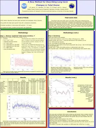
1. A New Method for Describing Long-term Changes in Total Ozone J. M. Harris1, S. J. Oltmans1, P. P. Tans1, R. D. Evans1, and D. L. Quincy2 1NOAA Climate Monitoring and Diagnostic Laboratory, Boulder, Colorado 80305 2Cooperative Institute for Research in the Environmental Sciences, University of Colorado, Boulder Results (cont.) Comparisons of total ozone tendency and growth rate curves: (a) midlatitude tendency curves for Bismarck (black), Nashville (green), Wallops Is. (blue), Boulder (gray), Caribou (purple), and Arosa (red). Tendency curves have been set to zero on July 1967 (the beginning of the shortest record) to aid the comparison; (b) growth rate curves for four coherent midlatitude sites using the same colors as above; (c) growth rate curves for the tropical sites, Samoa (light blue), Mauna Loa (orange) and Huancayo (pink). • Goals of Study • To be able to describe the total ozone decrease and (probable) future recovery. • To quantify the total ozone growth rate with a statistical uncertainty. • To detect variations in total ozone with periods > 3.5 years. • To visualize the data, tendency and growth rate graphically. Total ozone data The Dobson total ozone data used in this study (Table) were measured at five midlatitude sites and three tropical sites maintained and calibrated by the NOAA/Climate Monitoring and Diagnostics Laboratory. In addition, the Dobson total ozone data for Arosa, Switzerland were analyzed over two periods: July 1967 - November 2000 and July 1926 – November 2000. These data sets are archived at the World Ozone and Ultraviolet Radiation Data Centre in Downsview, Ontario, Canada. Total ozone monthly means were used in the analysis. Outliers in the data set were retained. Methodology Step 1. Remove ‘explained’ total ozone variation, Y Autoregressive model of total ozone (order 1 or 2): Y = constant 1Reconstructed solar irradiance from 200-295 nm: + b1x + b2x2 + b3x3 Lean, J., Evolution of the Sun’s spectral irradiance + seasonal harmonic terms since the Maunder minimum, Geophys. Res. Lett., + b4 * solar index1 27, 2425-2428, 2000. + b5 * temperature at 100 hPa2 2Kalnay et al., The NCEP/NCAR Reanalysis 40-year + b6 * temperature at 500 hPa2 project, Bull. Amer. Meteor. Soc. 77, 437-471, 1996. + b7 * QBO index3 3Randel,W. J., F. Wu, J. M. Russell III, J. W. Waters, + auto correlated noise and L. Froidevaux, Ozone and temperature changes inthe stratosphere following the eruption of Mount Pinatubo,J. Geophys. Res., 100, 16,753-16,764, 1995. Total ozone monthly means (diamonds) and AR fit of explained variation (red curve) for Bismarck, North Dakota. • Methodology (cont.) • Step 2. Bootstrap • Add cubic back to AR residuals. • Fit total ozone tendency curve (3.5-yr filter) [Thoning et al., 1989]. • Obtain growth rate curve = numerical derivative of the tendency curve. • Form 100 bootstrap samples. • Form 100 tendency and growth rate curves. • Uncertainty at each point on the trend and growth rate curves = SD of 100 bootstrap curves at that point. • Growth rate = mean of monthly points on initial growth rate curve. • SE of growth rate = SD about average of the 100 bootstrap mean growth rates. • Bismarck total ozone tendency curve Bismarck growth rate curve and 95% • (solid line) with 95% confidence limits confidence limits. • (dashed line). Residuals combined with • the cubic function from the AR fit are • shown as plus signs. Results Arosa total ozone tendency curve (solid line) with 95% confidence limits (dashed lines). Residuals combined with the cubic function from the AR fit are shown as plus signs. These points and the tendency curve have been adjusted so that the tendency curve starts at zero. • Conclusions • This new way to analyze total ozone tendencies and growth rates is better suited to describing both the total ozone decline and a potential future recovery. The curves used to track the total ozone tendency and growth rate are more flexible than the traditional linear trends. • Negative growth rates started in the 1970s. • Recovery from chemical depletion is not evident at the sites analyzed here. • Some stations show an unexplained coherence spanning the entire record, on a 4-12 year time scale. • The pattern of growth rate variations at SMO leads that of MLO by 1-2 years. • jharris@cmdl.noaa.gov