Distance Methods
Distance Methods. Distance Methods. Distance Estimates attempt to estimate the mean number of changes per site since 2 species (sequences) split from each other

Distance Methods
E N D
Presentation Transcript
Distance Methods • Distance Estimates attempt to estimate the mean number of changes per site since 2 species (sequences) split from each other • Simply counting the number of differences (p distance) may underestimate the amount of change - especially if the sequences are very dissimilar - because of multiple hits • We therefore use a model which includes parameters which reflect how we think sequences may have evolved
Some common models of sequence evolution commonly used in distance analysis: • Note that distance models are often based upon some of the same assumptions as the models in ML but they are implemented in a different way • Jukes Cantor model: assumes all changes equally likely • General time reversable model (GTR): assigns different probabilities to each type of change • LogDet / Paralinear distance model: was devised to deal with unequal base frequencies in different sequences • All of these models include a correction for multiple substitutions at the same site • All (except Logdet/paralinear distances) can be modified to include a gamma correction for site rate heterogeneity
A gamma distribution can be used to model site rate heterogeneity
The simplest model is that of Jukes & Cantor:dxy = -(3/4) ln (1-4/3 D) • dxy= distance between sequence x and sequence y expressed as the number of changes per site • (note dxy= r/n where r is number of replacements and n is the total number of sites. This assumes all sites can vary and when unvaried sites are present in two sequences it will underestimate the amount of change which has occurred at variable sites) • D = is the observed proportion of nucleotides which differ between two sequences (fractional dissimilarity) • ln = natural log function to correct for superimposed substitutions • The 3/4 and 4/3 terms reflect that there are four types of nucleotides and three ways in which a second nucleotide may not match a first - with all types of change being equally likely (i.e. unrelated sequences should be 25% identical by chance alone)
1 3 2 C G T A C A 1 Multiple changes at a single site - hidden changes Seq 1 AGCGAG Seq 2 GCGGAC Number of changes Seq 1 Seq 2
The natural logarithm ln is used to correct for superimposed changes at the same site • If two sequences are 95% identical they are different at 5% or 0.05 (D) of sites thus: • dxy = -3/4 ln (1-4/3 0.05) = 0.0517 • Note that the observed dissimilarity 0.05 increases only slightly to an estimated 0.0517 - this makes sense because in two very similar sequences one would expect very few changes to have been superimposed at the same site in the short time since the sequences diverged apart • However, if two sequences are only 50% identical they are different at 50% or 0.50 (D) of sites thus: • dxy = -3/4 ln (1-4/3 0.5) = 0.824 • For dissimilar sequences, which may diverged apart a long time ago, the use of ln infers that a much larger number of superimposed changes have occurred at the same site
A four taxon problem for Deinococcus and Thermus • Aquifex and Bacillus are thermophiles and mesophiles, respectively • No data suggest that Aquifex and Bacillus are specifically related to either Deinococcus or Thermus • If all four bacteria are included in an analysis the true tree should place Thermus and Deinococcus together Thermus Aquifex “The true tree” Deinococcus Bacillus
Comparison of observed (p) distances between sequences and JC distances for the same sequences using PAUP Uncorrected ("p") distance matrix 2 4 5 6 2 Aquifex - 4 Deinococc 0.25186 - 5 Thermus 0.18577 0.16866 - 6 Bacillus 0.21077 0.18881 0.19231 - Jukes-Cantor distance matrix 2 4 5 6 2 Aquifex - 4 Deinococc 0.30689 - 5 Thermus 0.21346 0.19106 - 6 Bacillus 0.24745 0.21751 0.22221 - Both distances give the incorrect tree Note that the JC distances are larger due to the correction for multiple substitutions
The 16S rRNA genes of Aquifex, Bacillus, Deinococcus and Thermus Exclude characters command in PAUP - exclude constant sites: Character-exclusion status changed: 859 of 1273 characters excluded Total number of characters now excluded = 859 Number of included characters = 414 Does the JC model fit these data? Base frequencies command in PAUP: Taxon A C G T # sites -------------------------------------------------------------- Aquifex 0.12319 0.38164 0.38164 0.11353 414 Deinococc 0.23188 0.22222 0.27295 0.27295 414 Thermus 0.13317 0.35835 0.37530 0.13317 413 Bacillus 0.23188 0.22705 0.26570 0.27536 414 -------------------------------------------------------------- Mean 0.18006 0.29728 0.32387 0.19879 413.75
Distance models can be made more parameter rich to increase their realism 1 • It is better to use a model which fits the data than to blindly impose a model on data • The most common additional parameters are: • A correction for the proportion of sites which are unable to change • A correction for variable site rates at those sites which can change • A correction to allow different substitution rates for each type of nucleotide change • PAUP will estimate the values of these additional parameters for you
Estimation of model parameters using maximum likelihood • Yang (1995) has shown that parameter estimates are reasonably stable across tree topologies provided trees are not “too wrong”. Thus one can obtain a tree using parsimony and then estimate model parameters on that tree. These parameters can then be used in a distance analysis (or a ML analysis).
Parameter estimates using the “tree scores” command in PAUP* Use PAUP* tree scores to use ML to estimate overthis tree: 1) Proportion of invariant sites 2) Gamma shape parameter for variable sites Tree number 1: -Ln likelihood = 4011.82617 Estimated value of proportion of invariable sites = 0.315477 Estimated value of gamma shape parameter = 0.501485 Maximum parsimony tree
Distance models can be made more parameter rich to increase their realism 2 JC -invariant sites + gamma correction for variable sites JC JC - invariant sites GTR-inv + gamma
The logDet/paralinear distances method 1 • LogDet/paralinear distances was designed to deal with unequal base frequencies in each pairwise sequence comparison - thus it allows base compositions to vary over the tree! • This distinguishes it from the GTR distance model which takes the average base composition and applies it to all comparisons
The logDet/paralinear distances method 2 • LogDet/paralinear distances assume all sites can vary - thus it is important to remove those sites which cannot change - this can be estimated using ML • Invariant sites are removed according to the base composition of constant sites (rather than the base composition of all sites - which may be different) in order to preserve the correct base frequencies among remaining constant sites
LogDet/Paralinear Distances dxy = -ln (det Fxy) • dxy= estimated distance between sequence x and sequence y • ln = natural log function to correct for superimposed substitutions • Fxy= 4 x 4 (there are four bases in DNA) divergence matrix for seq X & Y - this matrix summarises the relative frequencies of bases in a given pairwise comparison • det = is the determinant (a unique mathematical value) of the matrix
LogDet - a worked example for two sequences A and B Sequence B a c g t a 224 5 24 8 Sequence Ac 3 149 1 16 g 24 5 230 4 t 5 19 8 175 • For sequences A and B, over 900 sequence positions, this matrix summarises pairwise site by site comparisons (it uses the data very efficiently) • The matrix Fxy expresses this data as the proportions (e.g. 224/900 = 0.249) of sites: a c g t a .249 .006 .027 .009 Fxy = c .003 .166 .001 .018 g .027 .006 .256 .004 t .006 .021 .009 .194 • Dxy = -ln [det Fxy] = -ln [.002] = 6.216 (the LogDet distance between sequences A and B)
The logDet/paralinear distances method finds the true tree for Deinococcus + Thermus At last!
The logDet/paralinear distances method: advantages • Very goodfor situations where base compositions vary between sequences • Even when base compositions do not appear to vary the LogDet/Paralinear distances model performs at least as well as other distance methods • A drawback is that it assumes rates are equal for all sites • However, a correctionwhereby a proportion of invariable sites are removed prior to analysis appears to work very well as a “rate correction”
Distances: advantages: • Fast - suitable for analysing data sets which are too large for ML • A large number of models are available with many parameters - improves estimation of distances • Use ML to test the fit of model to data
Distances: disadvantages: • Information is lost - given only the distances it is impossible to derive the original sequences • Only through character based analyses can the history of sites be investigated e,g, most informative positions be inferred. • Generally outperformed by Maximum likelihood methods in choosing the correct tree in computer simulations (but LogDet can perform better than ML when base compositions vary)
Numbers of possible trees for N taxa: • For 10 taxa there are 2 x 10⁶ unrooted trees • For 50 taxa there are 3 x 1074 unrooted trees • How can we find the best tree ?
Obtaining a tree using pairwise distances Additive distances: • If we could determine exactly the true evolutionary distance implied by a given amount of observed sequence change, between each pair of taxa under study, these distances would have the useful property of tree additivity
C A 0.1 0.2 0.3 0.1 0.6 D B A perfectly additive tree A B C D A - 0.4 0.4 0.8 B 0.4 - 0.6 1.0 C 0.4 0.6 - 0.8 D 0.8 1.0 0.8 - The branch lengths in the matrix and the tree path lengths match perfectly - there is a single unique additive tree
Distance estimates may not make an additive tree Aquifex > Bacillus (0.335) Some path lengths are longer and others shorter than appear in the matrix Aquifex > Thermus (0.33) Jukes-Cantor distance matrix Proportion of sites assumed to be invariable = 0.56; identical sites removed proportionally to base frequencies estimated from constant sites only 1 2 4 5 6 1 ruber - 2 Aquifex 0.38745 - 4 Deinococc 0.22455 0.47540 - 5 Thermus 0.13415 0.273130.23615 - 6 Bacillus 0.27111 0.33595 0.28017 0.28846 - Thermus > Deinococcus (0.218)
Obtaining a tree using pairwise distances • Stochastic errors will cause deviation of the estimated distances from perfect tree additivity even when evolution proceeds exactly according to the distance model used • Poor estimates obtained using an inappropriate model will compound the problem • How can we identify the tree which best fits the experimental data from the many possible trees
Obtaining a tree using pairwise distances • We have uncertain data that we want to fit to a tree and find the optimal value for the adjustable parameters (branching pattern and branch lengths) • Use statistics to evaluate the fit of tree to the data (goodness of fit measures) • Fitch Margoliash method - a least squares method • Minimum evolution method - minimises length of tree • Note that neighbor joining while fast does not evaluate the fit of the data to the tree
Fitch Margoliash Method 1968: • Minimises the weighted squared deviation of the tree path length distances from the distance estimates
Fitch Margoliash Method 1968: Tree 2 - best Tree 1 Optimality criterion = distance (weighted least squares with power=2) Score of best tree(s) found = 0.12243 (average %SD = 11.663) Tree # 1 2 Wtd. S.S. 0.13817 0.12243 APSD 12.391 11.663
Minimum Evolution Method: • For each possible alternative tree one can estimate the length of each branch from the estimated pairwise distances between taxa and then compute the sum (S) of all branch length estimates. The minimum evolution criterion is to choose the tree with the smallest S value
Minimum Evolution Tree 2 Tree 1 - best Optimality criterion = distance (minimum evolution) Score of best tree(s) found = 0.68998 Tree # 1 2 ME-score 0.68998 0.69163