Download
1 / 42
420 likes | 582 Vues
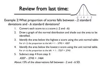
-2. -1. 0. 1. 2. Review from last time:. Example 2: What proportion of scores falls between -.2 standard deviations and -.6 standard deviations? Convert each score to a z score (-.2 and -.6) Draw a graph of the normal distribution and shade out the area to be identified.

E N D
-2 -1 0 1 2 Review from last time: Example 2: What proportion of scores falls between -.2 standard deviations and -.6 standard deviations? • Convert each score to a z score (-.2 and -.6) • Draw a graph of the normal distribution and shade out the area to be identified. • Identify the area below the highest z score using the unit normal table: For z=-.2, the proportion to the left = 1 - .5793 = .4207 • Identify the area below the lowest z score using the unit normal table. For z=-.6, the proportion to the left = 1 - .7257 = .2743 • Subtract step 4 from step 3: .4207 - .2743 = .1464 About 15% of the observations fall between -.2 and -.6 SD.
Probability & Samples: Distribution of Sample Means To recap… We recently learned how to convert a distribution of raw scores into a distribution of z-scores, and vice versa. We reviewed some basic probability concepts and observed how these apply to scores and distributions. Next we will learn about how to apply probability concepts to the binomial distribution (chapter 6), and to the distribution of sample means (chapter 7). Questions before we move on?
Binomial Distribution Number of heads HHH 3 HHT 2 HTH 2 HTT 1 2 THH THT 1 TTH 1 TTT 0 = 23 = 8total outcomes 2n
Binomial Distribution .4 .3 probability .2 .1 .125 .375 .375 .125 0 1 2 3 Number of heads Number of heads Distribution of possible outcomes (n = 3 flips) 3 2 2 1 2 1 1 0
Binomial Distribution Can make predictions about likelihood of outcomes based on this distribution. Distribution of possible outcomes (n = 3 flips) .4 What’s the probability of flipping three heads in a row? .3 probability .2 .1 p = 0.125 .125 .375 .375 .125 0 1 2 3 Number of heads
Binomial Distribution Can make predictions about likelihood of outcomes based on this distribution. Distribution of possible outcomes (n = 3 flips) .4 What’s the probability of flipping at least two heads in three tosses? .3 probability .2 .1 p = 0.375 + 0.125 = 0.50 .125 .375 .375 .125 0 1 2 3 Number of heads
Binomial Distribution Can make predictions about likelihood of outcomes based on this distribution. Distribution of possible outcomes (n = 3 flips) .4 What’s the probability of flipping all heads or all tails in three tosses? .3 probability .2 .1 p = 0.125 + 0.125 = 0.25 .125 .375 .375 .125 0 1 2 3 Number of heads
Binomial Distribution • Two categories of outcomes (A, B) (e.g., coin toss) • p=p(A)=Probability of A (e.g., Heads) • q=p(B) = Probability of B (e.g., Tails) • p + q = 1.0 (e.g., .5 + .5; could be different values) • n = number of observations (e.g., coin tosses) • X = number of times category A occurs in a sample • If pn > 10 and qn > 10, X follows a nearly normal distribution with μ = pn and σ =
Binomial Distribution • If pn > 10 and qn > 10, X follows a nearly normal distribution with μ = pn and σ = • Coin toss example, p=.5, q=.5, x=number of heads • With three tosses,μ = 1.5 and σ = = .87 X=3,3,3,3,3,2,2,2,2,2,2,2,2,2,2,2,1,1,1,1,0,0,0,0,0,0, M = 1.58 s = 1.06
New Topic Sampling Distributions & The Central Limit Theorem
Central Limit Theorem (p. 205) • For any population with mean μ and standard deviation σ, the distribution of sample means for sample size n will approach a normal distribution with a mean of μ and a standard deviation of and will approach a normal distribution as n approaches infinity This theorem provides the conceptual foundation of most of the inferential statistics covered in this class. Today we will learn about what it means and why it makes sense. In the next class we will see how the Central Limit Theorem makes inferential statistics possible.
Central Limit Theorem (p. 205) • For any population with mean μ and standard deviation σ, the distribution of sample means for sample size n will approach a normal distribution with a mean of μ and a standard deviation of and will approach a normal distribution as n approaches infinity This theorem provides the conceptual foundation of most of the inferential statistics covered in this class. Today we will learn about what it means and why it makes sense. In the next class we will see how the Central Limit Theorem makes inferential statistics possible.
Hypothesis testing Can make predictions about likelihood of outcomes based on this distribution. Distribution of possible outcomes (of a particular sample size, n) • In hypothesis testing, we compare our observed samples with the distribution of possible samples (transformed into standardized distributions) • This distribution of possible outcomes is often Normally Distributed
Distribution of sample means So far, when we have used the unit normal table to decide how “unlikely” a particular score is, our “comparison distribution” has been a distribution of individual scores In social science research, we are usually interested in making inferences about a mean of a group of scores (not just one score). Comparison distribution is the distribution of all possible sample means of a given sample size (“distribution of sample means”for short)
Distribution of sample means A simple case Population: 2 4 6 8 • All possible samples of size n = 2 Assumption: sampling with replacement
Distribution of sample means A simple case Population: 2 4 6 8 mean mean mean 4 6 5 8 2 5 4 8 6 8 4 6 2 6 6 2 4 8 6 7 2 8 6 4 5 8 8 8 4 2 6 6 6 4 4 6 8 7 • All possible samples of size n = 2 There are 16 of them 2 2 2 2 4 3 4 5 3 4
Distribution of sample means 5 4 3 2 1 2 3 4 5 6 7 8 means In long run, the random selection of tiles leads to a predictable pattern mean mean mean 2 2 2 4 6 5 8 2 5 2 4 3 4 8 6 8 4 6 2 6 4 6 2 4 8 6 7 2 8 5 6 4 5 8 8 8 4 2 3 6 6 6 4 4 4 6 8 7
Distribution of sample means Sample problem: What is the probability of getting a sample with a mean of 6 or more? 5 4 3 2 1 2 3 4 5 6 7 8 means P(M > 6) = .1875 + .1250 + .0625 = 0.375 • Same as before, except now we’re asking about sample means rather than single scores
Distribution of sample means Distribution of sample means is a “virtual” distribution between the sample and population Population Sample Distribution of sample means
Properties of the distribution of sample means Shape If population is Normal, then the distribution of sample means will be Normal N > 30 • If the sample size is large (n > 30), the distribution of sample means will be normal regardless of shape of the population Distribution of sample means Population
The mean of the dist of sample means is equal to the mean of the population Distribution of sample means same numeric value different conceptual values Properties of the distribution of sample means • Center Population
Center The mean of the dist of sample means is equal to the mean of the population Consider our earlier example Properties of the distribution of sample means 5 4 3 2 1 2 3 4 5 6 7 8 means Population Distribution of sample means 2 4 6 8 2 + 4 + 6 + 8 4 2+3+4+5+3+4+5+6+4+5+6+7+5+6+7+8 16 μ= = 5 = = 5
Spread The standard deviation of the distribution of sample means depends on two things Standard deviation of the population (as the standard deviation of the population gets larger, the standard deviation of the distribution of sample means also gets larger) Sample size (as the sample size gets larger, the standard deviation of the distribution of sample means gets smaller – law of large numbers) Properties of the distribution of sample means
Spread Standard deviation of the population Properties of the distribution of sample means 3 X X X X X 2 2 μ 1 X 3 μ μ • The smaller the population variability, the closer the sample means are to the population mean
Spread Sample size μ Properties of the distribution of sample means n = 1 M
Spread Sample size Properties of the distribution of sample means μ n = 10 M
Spread Sample size Properties of the distribution of sample means μ n = 100 The larger the sample size the smaller the spread M
Spread Standard deviation of the population Sample size Putting them together we get the standard deviation of the distribution of sample means Properties of the distribution of sample means • Commonly called the standard error (= SE = SEM = σM) • Can be thought of as the reliability of sample means (that is consistency expected between different measurements of the mean)
Standard error The standard error is the average amount that you’d expect a sample (of size n) to deviate from the population mean In other words, it is an estimate of the error that you’d expect by chance (or by sampling) The standard error is similar to the standard deviation, but it is important to know the difference between the two, both conceptually and mathematically!!!
Distribution of sample means Keep your distributions straight by taking care with your notation Population Sample σ s μ M Distribution of sample means
Properties of the distribution of sample means All three of these properties of the distribution of sample means (shape, center, and spread) are combined to form the Central Limit Theorem • For any population with mean μ and standard deviation σ, the distribution of sample means for sample size n will approach a normal distribution with a mean of μ and a standard deviation of as n approaches infinity • (good approximation if n > 30).
Properties of the distribution of sample means All three of these properties of the distribution of sample means (shape, center, and spread) are combined to form the Central Limit Theorem • For any population with mean μ and standard deviation σ, the distribution of sample means for sample size nwill approach a normal distribution with a mean of μ and a standard deviation of as n approaches infinity • (good approximation if n > 30). The standard distribution of the distribution of sample means ( ) is the standard error!
Who came up with the CLT & why? • Developed over more than a century and attributed to several different mathematicians. • Abraham DeMoivre (early-mid 1700s): While studying “games of chance” discovered that “coin toss” probabilities follow the normal distribution. • Pierre-Simon Laplace (late 1700s-early 1800s): Expanded on DeMoivre’s work while trying to estimate (via probability distributions) sums of meteor inclination angles.
The Central Limit Theorem is Your Friend Do yourself a favor and MEMORIZE IT!!
The Central Limit Theorem is Your Friend • It helps us make inferences about sample statistics (e.g., means) • For example, it can help us determine how likely or unlikely a particular sample mean is, given what we know about the population parameters.
Probability & the Distribution of Sample Means • We can use the Central Limit Theorem to calculate z-scores associated with individual sample means (the z-scores are based on the distribution of all possible sample means). • Each z-score describes the exact location of its respective sample mean, relative to the distribution of sample means. • Since the distribution of sample means is normal, we can then use the unit normal table to determine the likelihood of obtaining a sample mean greater/less than a specific sample mean.
Probability & the Distribution of Sample Means • When using z scores to represent sample means, the correct formula to use is:
Probability & the Distribution of Sample Means • EXAMPLE: What is the probability of obtaining a sample mean greater than M = 60 for a random sample of n = 16 scores selected from a normal population with a mean of μ = 65 and a standard deviation of σ = 20? • M = 60; μ = 65; σ = 20; n = 16
Recently we reviewed • Z-Scores • Probability • The connection between probability and distributions of individual scores • How to use the unit normal table to find probabilities associated with z-scores
Today we reviewed • The binomial distribution • The Central Limit Theorem & distribution of sample means • The connection between probability and the distribution of sample means
Last topic before the exam: • Hypothesis testing (pulls together everything we’ve learned so far and applies it to testing hypotheses about about sample means).
Hypothesis testing • Example: Testing the effectiveness of a new memory treatment for patients with memory problems • Our pharmaceutical company develops a new drug treatment that is designed to help patients with impaired memories. • Before we market the drug we want to see if it works. • The drug is designed to work on all memory patients, but we can’t test them all (the population). • So we decide to use a sample and conduct an experiment. • Based on the results from the sample we will make conclusions about the population. • Next time we’ll find out exactly how to do this!