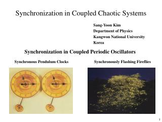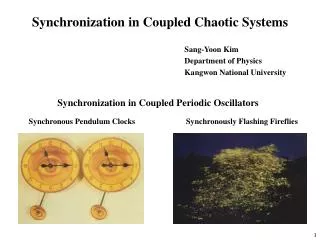
Synchronization of Chaotic Systems: Insights into Nonlinear Dynamics and Climate Prediction
This paper explores how two coupled chaotic systems can synchronize their dynamics through a single variable coupling, building upon the foundation laid by Pecora and Carroll in 1990. The study delves into the implications of synchronization in weather prediction and climate modeling, including the treatment of nonlinearities and parameter estimation. The authors present methods for optimal coupling in the presence of disturbances like white noise and address background error minimization. Insights into covariance inflation in data assimilation underline the role of nonlinearities in dynamic systems.

Synchronization of Chaotic Systems: Insights into Nonlinear Dynamics and Climate Prediction
E N D
Presentation Transcript
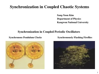
CHAOTIC SYSTEMS CAN SYNCHRONIZE DESPITE SENSITIVITY • two coupled chaotic systems can fall into synchronized motion along their strange attractors when linked through only one variable z (t) x’= (y-x) y’= x-y-xz z’= -z+xy y1’= x-y1-x(z1) z1’= -z1)+x(y1) (also works for y-coupling, but not for z-coupling) (Pecora and Carroll ’90)
SUPPOSE THE WORLD IS A LORENZ SYSTEM AND ONLY X IS OBSERVED • two coupled chaotic systems can fall into synchronized motion along their strange attractors when linked through only one variable z (t) x’= (y-x) y’= x-y-xz z’= -z+xy y1’= x-y1-x(z1) z1’= -z1)+x(y1) (also works for y-coupling, but not for z-coupling) (Pecora and Carroll ’90)
TWO CHANNEL MODELS SYNCHRONIZE WHEN DISCRETELY COUPLED - makes weather prediction possible “Truth” “Model” (Duane and Tribbia, PRL ’01, JAS ‘04)
Part I: Treatment of Nonlinearities in the Synchronization Approach Part II: Synchronization for Parameter Estimation, Model Learning and Fusion of Climate Models
Analysis: Synchronization with Noisy Coupling SDE’s: dxA/dt = f (xA) dxB/dt = f (xB) + C (xA- xB + ) is white noise < (t) T(t’) > = R d(t- t’) linearize: de/dt = Fe – Ce + C e xA- xB F Df(xA) Df(xB) Fokker-Planck eqn for PDF p(e): p/ t + e [p (F-C) e] = ½ t(CTRCp) Gaussian ansatz: p = N exp(-eTKe) pdne = 1 p/ t = 0 Choose C to minimize the spread B (2K)-1 of the distribution. Fluctuation-Dissipation Relation: B (C-F)T + (C-F) B = CRCT for C C + dC (dC arbitrary), let dB be such that B B + dB dB=0 if C= Copt = (1/ t) B R-1
Standard Data Assimilation As a Continuous Process (as in Einstein’s treatment of Brownian motion) Standard methods: xA=xbkd + [B(B+R)-1](xT - xbkd + noise) (perfect model) dxT/dt = f(xT) dxbkd/dt = f(xbkd) + (1/[B(B+R)-1](xT - xbkd + ) + O[ (B(B+R)-1)2] = f(xbkd) + (1/ BR-1 (xT - xbkd + ) is the time between analyses in incremental data assimilation The coupling C= (1/ t) B R-1 = Copt So, the standard methods of data assimilation (3DVar, Kalman Filtering) are also optimal for synchronization under local linearity assumption! (Exact treatment of discrete analysis cycle as a map gives Copt= (1/ t) B (B+R)-1. )
OPTIMAL COUPLING IN FULLY NONLINEAR CASE de/dt = (F-C)e + Cξ+ Ge2 + He3+ ξM ansatz: p=N exp(Ke2+Le3+Me4) Model error covariance Q=< ξM ξMT> p/ t + e [(F-C) e + Ge2 + He3]p = ½ t(CTRCp) In one dimension, Fokker-Planck eqn (F-C)e + Ge2 + He3 = ½ C2R (-2Ke – 3Le2 – 4Me3) F-C = ½ C2R (-2K) G = ½ C2R (-3L) H = ½ C2R (-4M) background error B= B(K,L,M) = ∫e2p(e)de = B(K(C),L(C),M(C)) optimize B as a function of C general correction to KF If we restrict form of C, e.g. C=F BR-1 cov. inflation factor F
f Choose G and H so that the dynamics are those of motion in a two-well potential: dx/dt = f (x) e.g. for d1,d2 matching the distances between the fixed points in the Lorenz ’84 system with F=1, one finds G = .15 H = -.75 Minimize background error B as a function of coupling C Find C = 1.51, B=0.145 B C If C = F B/(dR), then we have a covariance inflation factor F= 1.04 (where R=1, d = 0.1)
d1 No model error (Q=0): d2 d1 Model error equal to 50% of the resolved tendency: d2 The need for inflation is shaped by the nonlinearities, regardless of the amount of model error.
WHAT ABOUT SAMPLING ERROR? • Suppose undersampling uncertainty in estimate of B • multiplicative noise in assimilation dxT/dt = f(xT) dxbkd/dt = f(xbkd) + (1/[B(B+R)-1+ ξS](xT - xbkd + ) • Fokker Planck equation: • S2= =< ξS ξST> • p/ t + e [p (F-C + ½S2) e] • = ½ t2(CTRC+ S2 e2 - 2 Se/ (CTRC))p • Use change of variables p’= p(CTRC+ S2 e2 - 2 Se (CTRC)) • Arguably, effect is small if S< BR-1 • g
Multidimensional Case e.g. D=2 Consider two wells separated in one dimension. Assume R= (can arrange by rescaling) Choose a basis such that the dynamical equations are given by a direct product of motion in a two-well potential and simple linear dynamics. R is still diagonal. The FP equation p/ t + e [p (F-C) e] = ½ t(CTRCp) separates.
Summary: Covariance Inflation in the Synchronization Approach • In the synchronization approach, the rough magnitudes • of covariance inflation factors used in practice might be explained • from first principles • Model error due to unresolved physics makes little difference; the • requirement for inflation is shaped by nonlinearities in the dynamics • Refinements may yield treatments of nonlinearities that improve on • covariance inflation
Part I: Treatment of Nonlinearities in the Synchronization Approach Part II: Synchronization for Parameter Estimation, Model Learning and Fusion of Climate Models
WHAT IF THE MODEL IS IMPERFECT? • can synchronize parameters as well as states • Lorenz system example: • add parameter adaptation laws: r1’= (y-y1) x1 • n’ = (y1-y) y1 • m’= y-y1 x1’= (y-x1) y1’= 1x1- ny1-x1(z1)+m z1’= -z1)+x1(y1) x’= (y-x) y’= x-y-xz z’= -z+xy • these augmented equations minimize a Lyapunov function • V = ex2 + ey2 + ez2 + rr2+rn2+rm2 • where ex = x-x1, ey=……….. rr = r-r1, rn=……. • since it can be shown that dV/dt < 0, and V is bounded below • So as t→∞, (x1,y1,z1)→(x,y,z) and also r1→r, n→1, m→ 0 • i.e. the model “learns”
General Rule for Parameter Estimation, If Systems Synchronize with Identical Parameters dx/dt = f(x,p) dp/dt=0 dy/dt=f(y,q) + u(y,s) s=s(x) (30) dq/dt=N(y,x-y) (31) ey-x rq-p h f(y,q)- f(y,p) Truth: Model: (Duane , Yu, and Kocarev, Phys. Lett. A ‘06)
Example: A Column Model With an Unknown Surface Moisture Availability Parameter Column model summary:
Parameter Adaptation Rule Prognostic equation for humidity: nudging term soil moisture moisture availability parameter Adapt M according to: • interpretation: decrease or increase M in proportion to the • covariance between the synchronization (forecast) error and the • factor multiplied by M in the dynamical equations
RESULTS observations at 7 points in column nudging at 1 point nudging coeffiicient = .01 M-MT time -alternating periods of slow convergence to synchronization and rapid ``bursts” away -apparently can always identify the true value of M
….other configurations show same pattern observations and nudging at 7 points, coefficient = .0025 …as previous, but with nudging coefficient = .015 observations and nudging at 4 points, coefficient = .015 Actual details of model as implemented in software were unknown!
……..because the state variables also do not converge completely in the time interval shown qT qm
Single-Realization vs Ensembles • in principle, should be able to replace ensemble averages with • time averages to estimate relatively constant quantities • (cf. ergodicity) • “learn on the fly” → AI view of data assimilation • compare to “Lagged Average Forecasting” • (Hoffman and Kalnay ‘83 ): use a single realization with • different initialization times to create an artificial ensemble
Which parameters should we adapt? TAKE A COLLECTION OF THE BEST MODELS, COUPLE THEM TO ONE ANOTHER, AND ADAPT THE COUPLING COEFFICIENTS Ki constant: data assimilation adapt Clij: learning CONSENSUS -couple corresponding “model elements” l
Test Case: Fusing 3 Lorenz Systems With Different Parameters Average Output of Models (Unfused) z from Model With Best z Eqn Fused Models zMavg-zT zMbest-zT zMavg-zT not adapting Clij=0 adapting time time time dCxij/dt = a(xj-xi)(x – ⅓∑xk) dCyij/dt=……. dCzij/dt=……. - Model fusion is superior to any weighted averaging of outputs
Parameter Adaptation in the QG Channel Model What if foB ≠foB ? “model” B “truth ” A n=0 Add terms to FB to assimilate medium scales of A. Then adapt foB: foB’=∫(q*-qB)(qA-qB)d2x foB→foA timestep n
Proposed Adaptive Fusion of Different Channel Models Y* + Y*’ 2 forcing in Atlantic forcing in Pacific (k-dependence suppressed) Fo =fo(q-q*) Fo’=fo(q’-q*’) • If the parallel channels • synchronize, their common • solution also solves the • single-channel model with • the average forcing To find c adaptively: dc/dt = ∫d2x J(y,q’-q)(q-qobs) + ∫d2x J(y’,q-q’)(q’-qobs)
FUSION OF REAL CLIMATE MODELS Annual Mean SST Temperature COLA-MOM3 typical scenario: Observations oC CAM-MOM3 Longitude
SST CAM CAM_MOM3 Heat Flux Momentum Flux MOM
SST COLA COLA_MOM3 Heat Flux Momentum Flux MOM
SST CAM COLA Heat Flux Momentum Flux “Interactive Ensemble” MOM CAM_COLA_MOM3
SST CAM COLA Heat Flux “Interactive Ensemble” Momentum Flux MOM COLA_CAM_MOM3
Heat Flux: COLA; Momentum Flux: CAM Heat Flux: CAM; Momentum Flux: COLA
Observations COLA_MOM3 CAM_MOM3 Heat Flux: COLA; Momentum Flux: CAM Heat Flux: CAM; Momentum Flux: COLA
COLA_MOM3 CAM_MOM3 All Model Error Heat Flux: COLA; Momentum Flux: CAM Heat Flux: CAM; Momentum Flux: COLA
COLA_MOM3 CAM_MOM3 COLA Heat Flux Errors Heat Flux: COLA; Momentum Flux: CAM Heat Flux: CAM; Momentum Flux: COLA
COLA_MOM3 CAM_MOM3 Error Amplified by CAM Momentum Flux Heat Flux: COLA; Momentum Flux: CAM Heat Flux: CAM; Momentum Flux: COLA
COLA_MOM3 CAM_MOM3 CAM Heat Flux Error Heat Flux: COLA; Momentum Flux: CAM Heat Flux: CAM; Momentum Flux: COLA
INFERENCES ABOUT SOURCES OF ERROR WERE USED TO FORM A FUSED CAM-COLA MODEL Guiding principle: For each model element, make the choice of model that reduces truth-model synchronization error -simplified form of the automated adjustment of coupling coefficients (which need not be binary) proposed here
Adaptive Consensus Formation Approach is Empirical • -reminiscent of learning in neural networks: • Hebb’s rule: “Cells that fire together, wire together” • here: Model elements “wire together” directionally, • until they collectively ``fire” in sync with reality • Can the role of synchronization in the consensus formation scheme • be compared to its proposed role in consciousness, via the highly • intermittent synchronization of the 40 Hz oscillation in widely • separated regions of the brain?
Conclusion: Adaptive consensus formation among models can likely reduce error in long-range climate forecasts But what if the dynamical parameters change drastically in the 21st century as compared to the training period? Lorenz test case: Attractors Average of outputs (unfused) Fusion adaptation r=28 r=50 r=100 Other possible issues: -local vs. global optima in coupling coefficients -climate vs. weather prediction
Suggestive of Measure Synchronization…… • in jointly Hamiltonian systems, trajectories can become the same, • while states differ at any instant of time (Hampton & Zanette PRL ‘99) • Afraimovich et al. ‘97: “nonisochronic synchronization” of • dissipatively coupled systems: