Anomaly Detection Using Data Mining Techniques
Explore anomaly detection using event stream data mining techniques. Understand anomalies, modeling, and statistical views, with examples and visualizations. Learn about spatiotemporal data and time series stream modeling for dynamic insights.


Anomaly Detection Using Data Mining Techniques
E N D
Presentation Transcript
Anomaly Detection Using Data Mining Techniques Margaret H. Dunham, Yu Meng, Donya Quick, Jie Huang, Charlie Isaksson CSE Department Southern Methodist University Dallas, Texas 75275 mhd@engr.smu.edu This material is based upon work supported by the National Science Foundation under Grant No. IIS-0208741
Objectives/Outline Develop modeling techniques which can “learn/forget” past behavior of spatiotemporal stream events. Apply to prediction of anomalous events. • Introduction • EMM Overview • EMM Applications to Anomaly Detection • Future Work
Outline • Introduction • Motivation • What is an anomaly? • Spatiotemporal Data • Modeling Spatiotemporal Data • EMM Overview • EMM Applications to Anomaly Detection • Future Work
Motivation • A growing number of applications generate streams of data. • Computer network monitoring data • Call detail records in telecommunications • Highway transportation traffic data • Online web purchase log records • Sensor network data • Stock exchange, transactions in retail chains, ATM operations in banks, credit card transactions. • Data mining techniques play a key role in modeling and analyzing this data.
What is Anomaly? • Event that is unusual • Event that doesn’t occur frequently • Predefined event • What is unusual? • What is deviation?
What is Anomaly in Stream Data? • Rare - Anomalous – Surprising • Out of the ordinary • Not outlier detection • No knowledge of data distribution • Data is not static • Must take temporal and spatial values into account • May be interested in sequence of events • Ex: Snow in upstate New York is not an anomaly • Snow in upstate New York in June is rare • Rare events may change over time
Statistical View of Anomaly • Outlier • Data item that is outside the normal distribution of the data • Identify by Box Plot Image from Data Mining, Introductory and Advanced Topics, Prentice Hall, 2002.
Statistical View of Anomaly • Identify by looking at distribution • THIS DOES NOT WORK with stream data Image from www.wikipedia.org, Normal distribution.
Data Mining View of Anomaly • Classification Problem • Build classifier from training data • Problem is that training data shows what is NOT an anomaly • Thus an anomaly is anything that is not viewed as normal by the classification technique • MUST build dynamic classifier • Identify anomalous behavior • Signatures of what anomalous behavior looks like • Input data is identified as anomaly if it is similar enough to one of these signatures • Mixed – Classification and Signature
Visualizing Anomalies Temporal Heat Map (THM) is a visualization technique for streaming data derived from multiple sensors. • Two dimensional structure similar to an infinite table. • Each row of the table is associated with one sensor value. • Each column of the table is associated with a point in time. • Each cell within the THM is a color representation of the sensor value • Colors normalized (in our examples) • 0 – While • 0.5 – Blue • 1.0 - Red
THM of VoIP Data VoIP traffic data was provided by Cisco Systems and represents logged VoIP traffic in their Richardson, Texas facility from Mon Sep 22 12:17:32 2003 to Mon Nov 17 11:29:11 2003.
Spatiotemporal Stream Data • Records may arrive at a rapid rate • High volume (possibly infinite) of continuous data • Concept drifts: Data distribution changes on the fly • Data does not necessarily fit any distribution pattern • Multidimensional • Temporal • Spatial • Data are collected in discrete time intervals, • Data are in structured format, <a1, a2, …> • Data hold an approximation of the Markov property.
Spatiotemporal Environment • Events arriving in a stream • At any time, t, we can view the state of the problem as represented by a vector of n numeric values: Vt = <S1t, S2t, ..., Snt> Time
Data Stream Modeling • Single pass: Each record is examined at most once • Bounded storage: Limited Memory for storing synopsis • Real-time: Per record processing time must be low • Summarization (Synopsis )of data • Use data NOT SAMPLE • Temporal and Spatial • Dynamic • Continuous (infinite stream) • Learn • Forget • Sublinear growth rate - Clustering 11/26/07 – IRADSN’07 15
MM A first order Markov Chain is a finite or countably infinite sequence of events {E1, E2, … } over discrete time points, where Pij = P(Ej | Ei), and at any time the future behavior of the process is based solely on the current state A Markov Model (MM) is a graph with m vertices or states, S, and directed arcs, A, such that: • S ={N1,N2, …, Nm}, and • A = {Lij | i 1, 2, …, m, j 1, 2, …, m} and Each arc, Lij = <Ni,Nj> is labeled with a transition probability Pij = P(Nj | Ni).
Problem with Markov Chains • The required structure of the MC may not be certain at the model construction time. • As the real world being modeled by the MC changes, so should the structure of the MC. • Not scalable – grows linearly as number of events. • Our solution: • Extensible Markov Model (EMM) • Cluster real world events • Allow Markov chain to grow and shrink dynamically
Outline • Introduction • EMM Overview • EMM Applications to Anomaly Detection • Future Work
Extensible Markov Model (EMM) • Time Varying Discrete First Order Markov Model • Nodes are clusters of real world states. • Learning continues during application phase. • Learning: • Transition probabilities between nodes • Node labels (centroid/medoid of cluster) • Nodes are added and removed as data arrives
Related Work • Splitting Nodes in HMMs • Create new states by splitting an existing state • M.J. Black and Y. Yacoob,”Recognizing facial expressions in image sequences using local parameterized models of image motion”,Int. Journal of Computer Vision, 25(1), 1997, 23-48. • Dynamic Markov Modeling • States and transitions are cloned • G. V. Cormack, R. N. S. Horspool. “Data compression using dynamic Markov Modeling,”The Computer Journal, Vol. 30, No. 6, 1987. • Augmented Markov Model (AMM) • Creates new states if the input data has never been seen in the model, and transition probabilities are adjusted • Dani Goldberg, Maja J Mataric. “Coordinating mobile robot group behavior using a model of interaction dynamics,” Proceedings, the Third International Conference on Autonomous Agents (agents ’99), Seattle, Washington
EMM vs AMM Our proposed EMM model is similar to AMM, but is more flexible: • EMM continues to learn during the application phase. • The EMM is a generic incremental model whose nodes can have any kind of representatives. • State matching is determined using a clustering technique. • EMM not only allows the creation of new nodes, but deletion (or merging) of existing nodes. This allows the EMM model to “forget” old information which may not be relevant in the future. It also allows the EMM to adapt to any main memory constraints for large scale datasets. • EMM performs one scan of data and therefore is suitable for online data processing.
EMM Extensible Markov Model (EMM): at any time t, EMM consists of an MM and algorithms to modify it, where algorithms include: • EMMSim, which defines a technique for matching between input data at time t + 1 and existing states in the MM at time t. • EMMIncrement algorithm, which updates MM at time t + 1 given the MM at time t and classification measure result at time t + 1. Additional algorithms may be added to modify the model or for applications.
EMMSim • Find closest node to incoming event. • If none “close” create new node • Labeling of cluster is centroid/medoid of members in cluster • Problem • Nearest Neighbhor O(n) • BIRCH O(lg n) • Requires second phase to recluster initial
2/3 1/2 N3 2/3 N1 2/3 1/2 N3 1/3 1/1 N2 N1 N1 1/2 2/3 1/3 1/1 N2 1/3 N2 N1 1/3 N2 N3 1/1 1 N1 1/1 2/2 1/1 N1 EMMIncrement <18,10,3,3,1,0,0> <17,10,2,3,1,0,0> <16,9,2,3,1,0,0> <14,8,2,3,1,0,0> <14,8,2,3,0,0,0> <18,10,3,3,1,1,0.>
1/3 1/3 1/3 1/6 1/6 N1 N1 N3 N3 1/3 2/2 1/3 1/6 N2 1/3 1/2 N6 N6 N5 N5 EMMDecrement Delete N2
EMM Advantages • Dynamic • Adaptable • Use of clustering • Learns rare event • Scalable: • Growth of EMM is not linear on size of data. • Hierarchical feature of EMM • Creation/evaluation quasi-real time • Distributed / Hierarchical extensions
Growth of EMM Servent Data
EMM Performance – Growth Rate Minnesota Traffic Data
Outline • Introduction • EMM Overview • EMM Applications to Anomaly Detection • Future Work
Datasets/Anomalies • MnDot – Minnesota Department of Transportation • Automobile Accident • Ouse and Serwent – River flow data from England • Flood • Drought • KDD Cup’99 http://kdd.ics.uci.edu/databases/kddcup99/kddcup99.html • Intrusion • Cisco VoIP – VoIP traffic data obtained at Cisco • Unusual Phone Call
Rare Event Detection Detected unusual weekend traffic pattern Weekdays Weekend Minnesota DOT Traffic Data
Our Approach to Detect Anomalies • By learning what is normal, the model can predict what is not • Normal is based on likelihood of occurrence • Use EMM to build model of behavior • We view a rare event as: • Unusual event • Transition between events states which does not frequently occur. • Base rare event detection on determining events or transitions between events that do not frequently occur. • Continue learning
EMMRare • EMMRare algorithm indicates if the current input event is rare. Using a threshold occurrence percentage, the input event is determined to be rare if either of the following occurs: • The frequency of the node at time t+1 is below this threshold • The updated transition probability of the MC transition from node at time t to the node at t+1 is below the threshold
Determining Rare • Occurrence Frequency (OFc) of a node Nc : OFc = • Normalized Transition Probability (NTPmn), from one state, Nm, to another, Nn : NTPmn =
EMMRare Given: • Rule#1: CNi <= thCN • Rule#2: CLij <= thCL • Rule#3: OFc <= thOF • Rule#4: NTPmn <= thNTP Input: Gt: EMM at time t i: Current state at time t R= {R1, R2,…,RN}: A set of rules Output: At: Boolean alarm at time t Algorithm: At = 1 Ri = True 0 Ri = False
Risk assessment • Problem: Mitigate false alarm rate while maintaining a high detection rate. • Methodology: • Historic feedbacks can be used as a free resource to take out some possibly safe anomalies • Combine anomaly detection model and user’s feedbacks. • Risk level index • Evaluation metrics: Detection rate, false alarm rate. • Detection rate • False alarm rate • Operational Curve Detection rate = TP/(TP+TN) False alarm rate = FP/(TP+FP)
Reducing False Alarms Calculate Risk using historical feedback Historical Feedback: Count of true alarms:
Outline • Introduction • EMM Overview • EMM Applications to Anomaly Detection • Future Work
Ongoing/Future Work • Extend to Emerging Patterns • Extend to Hierarchical/Distributed • Yu Su • Test with more data – KDD Cup • Compare to other approaches • Charlie Isaksson • Apply to nuclear testing