Download

1 / 59
590 likes | 699 Vues
Explore the properties of algorithms, search and sorting techniques, and algorithmic paradigms in this comprehensive guide featuring examples and exercises. Discover how to effectively specify, analyze, and solve problems using algorithms. From defining algorithms to implementing them in pseudocode, this book covers critical concepts essential in the study of computational processes. Whether you are a student or a professional, this resource will deepen your understanding of algorithm complexity and its applications in various domains.

E N D
Algorithms Chapter 3 Sec 3.1 &3.2 With Question/Answer Animations
Chapter Summary • Algorithms • Example Algorithms • Algorithmic Paradigms • Growth of Functions • Big-O and other Notation • Complexity of Algorithms
Algorithms Section 3.1
Section Summary • Properties of Algorithms • Algorithms for Searching and Sorting • Greedy Algorithms • Halting Problem
Problems and Algorithms • In many domains, there are key general problems that ask for output with specific properties when given valid input. • The first step is to precisely state the problem, using the appropriate structures to specify the input and the desired output. • We then solve the general problem by specifying the steps of a procedure that takes a valid input and produces the desired output. This procedure is called an algorithm.
Algorithms Abu Ja’far Mohammed Ibin Musa Al-Khowarizmi (780-850) Definition: An algorithm is a finite sequence of precise instructions for performing a computation or for solving a problem. Example: Describe an algorithm for finding the maximum value in a finite sequence of integers. Solution: Perform the following steps: • Set the temporary maximum equal to the first integer in the sequence. • Compare the next integer in the sequence to the temporary maximum. • If it is larger than the temporary maximum, set the temporary maximum equal to this integer. • Repeat the previous step if there are more integers. If not, stop. • When the algorithm terminates, the temporary maximum is the largest integer in the sequence.
Specifying Algorithms • Algorithms can be specified in different ways. Their steps can be described in English or in pseudocode. • Pseudocode is an intermediate step between an English language description of the steps and a coding of these steps using a programming language. • The form of pseudocode we use is specified in Appendix 3. It uses some of the structures found in popular languages such as C++ and Java. • Programmers can use the description of an algorithm in pseudocode to construct a program in a particular language. • Pseudocode helps us analyze the time required to solve a problem using an algorithm, independent of the actual programming language used to implement algorithm.
Properties of Algorithms • Input: An algorithm usually has input values from a specified set. • Output: From the input values, the algorithm produces the output values from a specified set. The output values are the solution. • Correctness: An algorithm should produce the correct output values for each set of input values. • Finiteness: An algorithm should produce the output after a finite number of steps for any input. • Effectiveness: It must be possible to perform each step of the algorithm correctly and in a finite amount of time. • Generality: The algorithm should work for all problems of the desired form.
Finding the Maximum Element in a Finite Sequence • The algorithm in pseudocode: • Does this algorithm have all the properties listed on the previous slide? proceduremax(a1, a2, …., an: integers) max := a1 fori := 2 to n • ifmax < ai then max := ai • return max{max is the largest element}
Some Example Algorithm Problems • Three classes of problems will be studied in this section. • Searching Problems: finding the position of a particular element in a list. • Sorting problems: putting the elements of a list into increasing order. • Optimization Problems: determining the optimal value (maximum or minimum) of a particular quantity over all possible inputs.
Searching Problems Definition: The general searching problem is to locate an element x in the list of distinct elements a1,a2,...,an, or determine that it is not in the list. • The solution to a searching problem is the location of the term in the list that equals x (that is, iis the solution if x = ai) or 0if x is not in the list. • For example, a library might want to check to see if a patron is on a list of those with overdue books before allowing him/her to checkout another book. • We will study two different searching algorithms; linear search and binary search.
Linear Search Algorithm • The linear search algorithm locates an item in a list by examining elements in the sequence one at a time, starting at the beginning. • First compare x with a1. If they are equal, return the position 1. • If not, try a2. If x = a2, return the position 2. • Keep going, and if no match is found when the entire list is scanned, return 0. procedurelinearsearch(x:integer, a1, a2, …,an: distinct integers) i := 1 while (i≤n and x ≠ ai) i := i + 1 • ifi≤nthenlocation := i elselocation := 0 returnlocation{location is the subscript of the term that equals x, or is 0 if x is not found}
Binary Search • Assume the input is a list of items in increasing order. • The algorithm begins by comparing the element to be found with the middle element. • If the middle element is lower, the search proceeds with the upper half of the list. • If it is not lower, the search proceeds with the lower half of the list (through the middle position). • Repeat this process until we have a list of size 1. • If the element we are looking for is equal to the element in the list, the position is returned. • Otherwise, 0 is returned to indicate that the element was not found. • In Section 3.3, we show that the binary search algorithm is much more efficient than linear search.
Binary Search • Here is a description of the binary search algorithm in pseudocode. procedure binarysearch(x: integer, a1,a2,…, an: increasing integers) i := 1 {i is the left endpoint of interval} j := n {j is right endpoint of interval} whilei < j • m := ⌊(i + j)/2⌋ ifx > am then i := m + 1 elsej := m if x = aithenlocation := i else location := 0 returnlocation{location is the subscript i of the term ai equal to x, or 0 if x is not found}
Binary Search Example: The steps taken by a binary search for 19 in the list: 1 2 3 5 6 7 8 10 12 13 15 16 18 19 20 22 • The list has 16 elements, so the midpoint is 8. The value in the 8th position is 10. Since 19 > 10, further search is restricted to positions 9through 16. 1 2 3 5 6 7 8 10 12 13 15 16 18 19 20 22 • The midpoint of the list (positions 9 through 16) is now the 12th position with a value of 16. Since 19 > 16, further search is restricted to the 13th position and above. 1 2 3 5 6 7 8 1012 13 15 16 18 19 20 22 • The midpoint of the current list is now the 14th position with a value of 19. Since 19 ≯ 19, further search is restricted to the portion from the 13th through the 14th positions . 1 2 3 5 6 7 8 1012 13 15 16 18 19 20 22 • The midpoint of the current list is now the 13th position with a value of 18. Since 19> 18, search is restricted to the portion from the 18th position through the 18th. 1 2 3 5 6 7 8 1012 13 15 16 18 19 20 22 • Now the list has a single element and the loop ends. Since 19=19, the location 16 is returned.
Big Mantra of Algorithm Efficiency • You can usually come up with a faster algorithm if you are willing to place restrictions on the types of inputs that it can handle • Linear Search (Slower) • Works with ANY list • Binary Search (Faster) • Only works with SORTED lists
Sorting • To sort the elements of a list is to put them in increasing order (numerical order, alphabetic, and so on). • Sorting is an important problem because: • A nontrivial percentage of all computing resources are devoted to sorting different kinds of lists, especially applications involving large databases of information that need to be presented in a particular order (e.g., by customer, part number etc.). • An amazing number of fundamentally different algorithms have been invented for sorting. Their relative advantages and disadvantages have been studied extensively. • Sorting algorithms are useful to illustrate the basic notions of computer science. • A variety of sorting algorithms are studied in this class; binary, insertion, bubble, selection, merge, quick, and tournament. • In Section 3.3, we’ll study the amount of time required to sort a list using the sorting algorithms covered in this section.
SelectionSort • Selection sort makes multiple passes through a list. On every passithe ith largest element is placed in the ith position procedureselectionsort(a1,…,an: real numbers with n≥2) fori:= 1 to n− 1 • max := i • for j := i+1 to n • if (aj > amax)then max := j • interchange aiwith amax • {a1,…, an is now in decreasing order}
Bubble Sort • Bubble sort makes multiple passes through a list. Every pair of elements that are found to be out of order are interchanged. procedurebubblesort(a1,…,an: real numbers with n≥2) fori:= 1 to n− 1 • for j := 1 to n − i ifaj >aj+1then interchange aj and aj+1 {a1,…, an is now in increasing order}
Bubble Sort Example: Show the steps of bubble sort with 3 2 4 1 5 • At the first pass the largest element has been put into the correct position • At the end of the second pass, the 2nd largest element has been put into the correct position. • In each subsequent pass, an additional element is put in the correct position.
Insertion Sort • Insertion sort begins with the 2nd element. It compares the 2nd element with the 1st and puts it before the first if it is not larger. procedureinsertionsort (a1,…,an: real numbers with n≥2) for j := 2 to n i := 1 whileaj > ai i := i + 1 m := aj • fork := 0 to j−i− 1 aj-k := aj-k-1 ai := m {Now a1,…,anis in increasing order} • Next the 3rd element is put into the correct position among the first 3 elements. • In each subsequent pass, the n+1st element is put into its correct position among the first n+1 elements. • Linear search is used to find the correct position.
Insertion Sort Example: Show all the steps of insertion sort with the input: 3 2 4 1 5 • 2 3 4 1 5 (first two positions are interchanged) • 2 34 1 5 (third element remains in its position) • 1 2 34 5 (fourth is placed at beginning) • 1 2 345 (fifth element remains in its position)
Greedy Algorithms • Optimization problems minimize or maximize some parameter over all possible inputs. • Among the many optimization problems we will study are: • Finding a route between two cities with the smallest total mileage. • Determining how to encode messages using the fewest possible bits. • Finding the fiber links between network nodes using the least amount of fiber. • Optimization problems can often be solved using a greedy algorithm, which makes the “best” choice at each step. Making the “best choice” at each step does not necessarily produce an optimal solution to the overall problem, but in many instances, it does. • After specifying what the “best choice” at each step is, we try to prove that this approach always produces an optimal solution, or find a counterexample to show that it does not. • The greedy approach to solving problems is an example of an algorithmic paradigm, which is a general approach for designing an algorithm. We return to algorithmic paradigms in Section 3.3.
Greedy Algorithms: Making Change Example: Design a greedy algorithm for making change (in U.S. money) of n cents with the following coins: quarters (25 cents), dimes (10 cents), nickels (5 cents), and pennies (1 cent) , using the least total number of coins. Idea: At each step choose the coin with the largest possible value that does not exceed the amount of change left. • If n = 67 cents, first choose a quarter leaving 67−25 = 42 cents. Then choose another quarter leaving 42 −25 = 17 cents • Then choose 1 dime, leaving 17 − 10 = 7 cents. • Choose 1 nickel, leaving 7 – 5 – 2 cents. • Choose a penny, leaving one cent. Choose another penny leaving 0 cents.
Greedy Change-Making Algorithm Solution: Greedy change-making algorithm for n cents. The algorithm works with any coin denominations c1, c2, …,cr. • For the example of U.S. currency, we may have quarters, dimes, nickels and pennies, with c1= 25, c2= 10, c3= 5, and c4= 1. • procedurechange(c1, c2, …, cr: values of coins, where c1> c2> … > cr; n:a positive integer) • for i := 1 to r • di:= 0 [dicounts the coins of denomination ci] whilen ≥ci • di := di + 1 [add a coin of denomination ci] • n=n -ci • [dicounts the coins ci]
Proving Optimality for U.S. Coins • Show that the change making algorithm for U.S. coins is optimal. Lemma 1: If n is a positive integer, then n cents in change using quarters, dimes, nickels, and pennies, using the fewest coins possible has at most 2 dimes, 1 nickel, 4 pennies, and cannot have 2 dimes and a nickel. The total amount of change in dimes, nickels, and pennies must not exceed 24 cents. Proof: By contradiction • If we had 3 dimes, we could replace them with a quarter and a nickel. • If we had 2 nickels, we could replace them with 1 dime. • If we had 5 pennies, we could replace them with a nickel. • If we had 2 dimes and 1 nickel, we could replace them with a quarter. • The allowable combinations, have a maximum value of 24 cents; 2 dimes and 4 pennies.
Proving Optimality for U.S. Coins Theorem: The greedy change-making algorithm for U.S. coins produces change using the fewest coins possible. Proof: By contradiction. • Assume there is a positive integer n such that change can be made for n cents using quarters, dimes, nickels, and pennies, with a fewer total number of coins than given by the algorithm. • Then, q̍≤ q where q̍ is the number of quarters used in this optimal way and q is the number of quarters in the greedy algorithm’s solution. But this is not possible by Lemma 1, since the value of the coins other than quarters can not be greater than 24 cents. • Similarly, by Lemma 1, the two algorithms must have the same number of dimes, nickels, and quarters.
Greedy Change-Making Algorithm • Optimality depends on the denominations available. • For U.S. coins, optimality still holds if we add half dollar coins (50 cents) and dollar coins (100 cents). • But if we allow only quarters (25 cents), dimes (10 cents), and pennies (1 cent), the algorithm no longer produces the minimum number of coins. • Consider the example of 31 cents. The optimal number of coins is 4, i.e., 3 dimes and 1 penny. What does the algorithm output?
Greedy Scheduling S.S. to Slide 29 Example: We have a group of proposed talks with start and end times. Construct a greedy algorithm to schedule as many as possible in a lecture hall, under the following assumptions: • When a talk starts, it continues till the end. • No two talks can occur at the same time. • A talk can begin at the same time that another ends. • Once we have selected some of the talks, we cannot add a talk which is incompatible with those already selected because it overlaps at least one of these previously selected talks. • How should we make the “best choice” at each step of the algorithm? That is, which talk do we pick ? • The talk that starts earliest among those compatible with already chosen talks? • The talk that is shortest among those already compatible? • The talk that ends earliest among those compatible with already chosen talks?
Greedy Scheduling S.S. to Slide 29 • Picking the shortest talk doesn’t work. • Can you find a counterexample here? • But picking the one that ends soonest does work. The algorithm is specified on the next page. Start: 8:00 AM Start: 9:00 AM Start: 9:45 AM Talk 1 Talk 2 Talk 3 End: 10:00 AM End :9:45 AM End: 11:00 AM
Greedy Scheduling algorithm S.S. to Slide 29 Solution: At each step, choose the talks with the earliest ending time among the talks compatible with those selected. • Will be proven correct by induction in Chapter 5. • procedureschedule(s1≤ s2≤ … ≤ sn:start times, e1≤ e2≤ … ≤ en :end times) • sort talks by finish time and reorder so that e1≤ e2≤ … ≤ en • S := ∅ • for j := 1 to n • if talk j is compatible with S then • S := S ∅∪{talk j} • return S [ S is the set of talks scheduled]
Halting Problem Example: Can we develop a procedure that takes as input a computer program along with its input and determines whether the program will eventually halt with that input. • Solution: Proof by contradiction. • Assume that there is such a procedure and call it H(P,I). The procedure H(P,I) takes as input a program P and the input I to P. • H outputs “halt” if it is the case that P will stop when run with input I. • Otherwise, H outputs “loops forever.”
Halting Problem • Since a program is a string of characters, we can call H(P,P). Construct a procedure K(P), which works as follows. • If H(P,P) outputs “loops forever” then K(P) halts. • If H(P,P) outputs “halt” then K(P) goes into an infinite loop printing “ha” on each iteration.
Halting Problem • Now we call K with K as input, i.e. K(K). • If the output of H(K,K) is “loops forever” then K(K) halts. A Contradiction. • If the output of H(K,K) is “halts” then K(K) loops forever. A Contradiction. • Therefore, there can not be a procedure that can decide whether or not an arbitrary program halts. The halting problem is unsolvable by an algorithm.
The Growth of Functions Section 3.2
Section Summary Donald E. Knuth (Born 1938) • Big-O Notation • Big-O Estimates for Important Functions • Big-Omega and Big-Theta Notation Edmund Landau (1877-1938) Paul Gustav Heinrich Bachmann (1837-1920)
The Growth of Functions • In both computer science and in mathematics, there are many times when we care about how fast a function grows. • In computer science, we want to understand how quickly an algorithm can solve a problem as the size of the input grows. • We can compare the efficiency of two different algorithms for solving the same problem. • We can also determine whether it is practical to use a particular algorithm as the input grows. • We’ll study these questions in Section 3.3. • Two of the areas of mathematics where questions about the growth of functions are studied are: • number theory (covered in Chapter 4) • combinatorics (covered in Chapters 6 and 8)
Big-O Notation Definition: Let f and g be functions from the set of integers or the set of real numbers to the set of real numbers. We say that f(x) is O(g(x)) if there are constants C and k such that whenever x > k. (illustration on next slide) • This is read as “f(x) is big-O of g(x)” or “g asymptotically dominates f.” • The constants C and k are called witnesses to the relationship f(x) is O(g(x)). Only one pair of witnesses is needed.
Illustration of Big-O Notation f(x) is O(g(x)
Some Important Points about Big-O Notation • If one pair of witnesses is found, then there are infinitely many pairs. We can always make the k or the C larger and still maintain the inequality . • Any pair C̍ and k̍ where C < C̍ and k < k ̍ is also a pair of witnesses since whenever x > k̍> k. You may see “ f(x) = O(g(x))” instead of “ f(x) is O(g(x)).” • But this is an abuse of the equals sign since the meaning is that there is an inequality relating the values of f and g, for sufficiently large values of x. • It is ok to write f(x) ∊O(g(x)), because O(g(x)) represents the set of functions that are O(g(x)). • Usually, we will drop the absolute value sign since we will always deal with functions that take on positive values.
Using the Definition of Big-O Notation Example: Show that is . Solution: Since when x > 1, x < x2 and 1 < x2 • Can take C = 4and k = 1 as witnesses to show that (see graph on next slide) • Alternatively, when x > 2, we have 2x≤x2 and 1 < x2. Hence, when x > 2. • Can take C = 3and k = 2 as witnesses instead.
Big-O Notation • Both and are such that and . We say that the two functions are of the same order. (More on this later) • If and h(x) is larger than g(x) for all positive real numbers, then . • Note that if for x > k and if for all x, then if x > k. Hence, . • For many applications, the goal is to select the function g(x) in O(g(x)) as small as possible (up to multiplication by a constant, of course).
Using the Definition of Big-O Notation Example: Show that 7x2 is O(x3). Solution: When x > 7, 7x2 < x3. TakeC=1 andk = 7 as witnesses to establish that 7x2 is O(x3). (WouldC = 7 andk = 1 work?) Example: Show that n2 is not O(n). Solution: Suppose there are constants C and k for which n2≤Cn, whenever n > k. Then (by dividing both sides of n2≤Cn) by n, then n≤C must hold for all n > k. A contradiction!
Big-O Estimates for Polynomials Example: Let where are real numbers with an ≠0. Then f(x) is O(xn). Proof: |f(x)| = |anxn+ an-1 xn-1 + ∙∙∙+ a1x1 + a1| ≤ |an|xn + |an-1| xn-1 + ∙∙∙+ |a1|x1+ |a1| = xn(|an| + |an-1| /x+ ∙∙∙+ |a1|/xn-1+ |a1|/xn) ≤ xn(|an| + |an-1| + ∙∙∙+ |a1|+ |a1|) • Take C = |an| + |an-1| + ∙∙∙+ |a1|+ |a1| and k = 1. Then f(x) is O(xn). • The leading term anxn of a polynomial dominates its growth. Uses triangle inequality, an exercise in Section 1.8. Assuming x > 1
Big-O Estimates for some Important Functions Example: Use big-O notation to estimate the sum of the first n positive integers. Solution: Example: Use big-O notation to estimate the factorial function Solution: Continued →
Big-O Estimates for some Important Functions Example: Use big-O notation to estimate log n! Solution: Given that (previous slide) then . Hence, log(n!) is O(n∙log(n)) taking C = 1 and k = 1.
Display of Growth of Functions Note the difference in behavior of functions as n gets larger
Useful Big-O Estimates Involving Logarithms, Powers, and Exponents • If d > c > 1, then ncis O(nd), but ndis not O(nc). • If b > 1 and c and d are positive, then (logb n)cis O(nd), but ndis not O((logb n)c). • If b > 1 and d is positive, then ndis O(bn), but bnis not O(nd). • If c > b > 1, then bnis O(cn), but cnis not O(bn).
Self Study Combinations of Functions • If f1 (x) is O(g1(x)) and f2 (x) is O(g2(x)) then ( f1 + f2 )(x) is O(max(|g1(x) |,|g2(x) |)). • See next slide for proof • If f1 (x) and f2 (x) are both O(g(x)) then ( f1 + f2 )(x) is O(g(x)). • See text for argument • If f1 (x) is O(g1(x)) and f2 (x) is O(g2(x)) then ( f1f2 )(x) is O(g1(x)g2(x)). • See text for argument