#3191, 14 Oct 2012
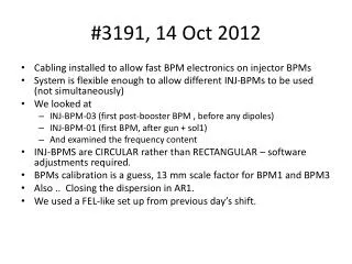
#3191, 14 Oct 2012 . Cabling installed to allow fast BPM electronics on injector BPMs System is flexible enough to allow different INJ-BPMs to be used (not simultaneously) We looked at INJ-BPM-03 (first post-booster BPM , before any dipoles) INJ-BPM-01 (first BPM, after gun + sol1)

#3191, 14 Oct 2012
E N D
Presentation Transcript
#3191, 14 Oct 2012 • Cabling installed to allow fast BPM electronics on injector BPMs • System is flexible enough to allow different INJ-BPMs to be used (not simultaneously) • We looked at • INJ-BPM-03 (first post-booster BPM , before any dipoles) • INJ-BPM-01 (first BPM, after gun + sol1) • And examined the frequency content • INJ-BPMS are CIRCULAR rather than RECTANGULAR – software adjustments required. • BPMs calibration is a guess, 13 mm scale factor for BPM1 and BPM3 • Also .. Closing the dispersion in AR1. • We used a FEL-like set up from previous day’s shift.
WARNING !!! • The y BPM data in this file is all incorrect due to software bug present at the time. • The code used to compute y was • The correct code should be • However the raw A, B, C, D data is still there in the file so all the data can be reconstructed (B-P2)-(D-P2)/((B-P2)+(D-P2)) ((B-P2)-(D-P2))/((B-P2)+(D-P2))
INJ-BPM-03 • Nominal FEL set-up. ‘Typical’ 1-shot BPM train measurement x (mm), y (mm), sum voltage Fourier transform vertical axis amplitude^2 horizontal axis frequency in MHz Fourier transforms done after subtracting mean values 100 KHz obvious in x y very similar to sum_pickup voltage 6 Mhz present, smaller than 100 KHz ‘usual’ 300 KHz present
Shot-by-shot variation • I THINK (not enough data to prove) that the DFT power spectrum might vary quite a bit from train to train • The variation might be big enough to obscure some effects when trying to judge effect of scanning each accelerator param • i.e. is the parameter (magnet strength etc) changing the DFT, or is the DFT changing in time anyway?
INJ-BPM-03 Buncher OFF • On EVERY shot with buncher OFF, the x trace is a lot ‘hairier’ than with buncher ON 6 MHz looks enhanced ‘hairier’ and fourier confirms. But 100 kHz also enhanced
Any 100 kHz in y ? • Another shot with nominal set-up Some 100 kHz in y here.
Other Parameters Variation on BPM3 • We varied several other injector parameters (apart from buncher power) • 2 quads between booster and BPM3 • Booster entrance correctors. • Solenoids • General, crude observations • No parameter enhanced 100 kHz (some suppressed it very strongly) • SOL-02 seemed to enhance the 6 MHz the most
INJ-BPM-01 • Took 1 shot as a reference Note scale change here Is there 100 KHz here or not?
Parameters Variation on BPM1 • Varied HVCOR-01, SOL-01, and Gun HV (changed to 230 kV, rather arbitrarily) • Crude observations again • Difficult to see 100 kHz, but perhaps it is there (I see small peak on y on some of the shots) • Gun HV didn’t seem to drastically change the frequency content of x, y, charge • 6 MHz stronger on x than y generally.
Other observations • The amplitudes of the frequency components vary shot to shot. • Need to be careful when changing parameters and concluding “this parameter enhances the oscillation at X Mhz”, you can probably trick yourself into observing effects.
General Conclusions • I think there is enough evidence here to say that the 100 kHz seen in AR1 (on x AND y) cannot be solely due to ALICE dipoles (as PHW simulated). 100 KHz comes certainly in injector before any dipoles. • Y is very similar to SUM_CHARGE.
Dispersion at AR1 Exit • Use AR1-BPM-06 and measure x/E for different AR1Q1/4 values ERROR, DUPLICATED DATA Despite the error, the closed arc condition can be interpolated
FCUP-01 Frequency Analysis • Record FCUP-01 trace using high-res scope (20 Gsamples/sec == 1 sample every 50 ps) • 100 uS bunch train == 100 Mbytes. Mathematica has problems with this size of data • Took 1 in every 10 points (1 sample every 0.5 ns) to help things. • The DFT frequency spectrum ranges from 10 kHz to 1 GHz, although only part of this spectrum is meaningful due to fcup time response • However, you can see the individual bunches on the scope! • To do DFT, first take off similar transient to the transients we have been removing in BPM DFT (100 bunches ~ 6 μs) • Then subtract mean charge and perform DFT 16 humps in 1 μs == 16 MHz, these are the bunches
FCUP-01 Frequency Analysis Various regions of the frequency spectrum Horizontal axis is in Hz in all plots Bunch frequency 16 MHz + harmonics due to “triangle” shape of bunches on FCUP 6MHz we have seen in the BPM charge signal and x and y Bunch frequency 16 MHz This is also an artefact of the 6MHz, it is the sideband 16 MHZ – 6 MHz. i.e. the envelope 6MHz we have seen in the BPM charge signal and x and y 300 kHz we have seen in the BPM charge signal and x and y
FCUP-01 Frequency Analysis 300 kHz we have seen in the BPM charge signal and x and y No 100 kHz visible Compare with IBIC data from #3121 Fourier transform of summed ARC1 BPM signal MHz If 100 kHz (seen on the BPM x signals) was electrical noise on the cables, wouldn’t it be visible in both the FCUP signal and the BPM individual button voltage signals?