Detecting Periodicity in Point Processes
250 likes | 272 Vues
This research paper discusses the challenges in detecting periodicity in point processes, specifically focusing on the identification of periodic gamma-ray sources. The paper explores various score tests and their significance in blind searches, highlighting the need for empirical comparisons. It also examines the computational demands and limitations of blind searches in order to provide insights into developing effective detection algorithms. The paper concludes with a discussion on the use of classical extreme value theory in conjunction with affordable simulations for assessing significance.

Detecting Periodicity in Point Processes
E N D
Presentation Transcript
Detecting Periodicity in Point Processes • John Rice • University of California, Berkeley • “All animals act as if they can make decisions.” (I. J. Good) • Joint work with Peter Bickel and Bas Kleijn. Thanks to Seth Digel, Patrick Nolan and Tom Loredo
Outline Introduction and motivation A family of score tests Assessing significance in a blind search The need for empirical comparisons
Motivation Many gamma-ray sources are unidentified and may be pulsars, but establishing that these sources are periodic is difficult. Might only collect ~1500 photons during a 10 day period.
Difficulties Frequency unknown Spins down Large search space Glitches Celestial foreground Computational demands for a blind search are very substantial. A heroic search did not find any previously unknown gamma-ray pulsars in EGRET data. (Chandler et al, 2001).
Unpleasant fact:There is no optimal test.A detection algorithm optimal for one function will not be optimal for another function. No matter how clever you are, no matter how rich the dictionary from which you adaptively compose a detection statistic, no matter how multilayered your hierarchical prior, your procedure will not be globally optimal. The pulse profile (t) is an infinite dimensional object. Any test can achieve high asymptotic power against local alternatives for at most a finite number of directions. In other words, associated with any particular test is a finite dimensional collection of targets and it is only for such targets that it is highly sensitive. Consequence: You have to be a [closet] Bayesian and choose directions a priori. Lehman & Romano. Testing Statistical Hypotheses. Chapt 14
Likelihood function and score test • Let the point spread function be w(z|e). The likelihood given times (t), energies (e), and locations (z) of photons: where wj =w(zj | ej).. A score test (Rao test) is formed by differentiating the log likelihood with respect to and evaluating the derivative at = 0: Neglible if period << T Unlike a generalized ratio test, a Rao test does not require fitting parameters under the alternative, but only under the null hypothesis.
Phase invariant statistic • Square and integrate out phase. Neglecting the second term: • Apart from psf-weighting was proposed by Beran as locally most powerful invariant test in the direction ( ) at frequency f. Truncating at n=1 gives Rayleigh test. Truncating at n=M gives ZM2. Particular choice of coefficients gives Watson’s test (invariant form of Cramer-von Mises). Mardia (1972). Statistics of Directional Data
Relationship to tests based on density estimation • In the unweighted case the test statistic can be expressed as • A continuous version of a chi-square goodness of fit test using kernel density estimate rather than binning. But note that a kernel for density estimation is usually taken to be sharply peaked and thus have substantial high frequency content! Such a choice of ( ) will not match low frequency targets. Kernel density estimate
Power • Let • And suppose the signal is • and • Then
Tradeoffs • The n-th harmonic will only contribute to the power if n is substantial and if nis small. That is, inclusion of harmonics is only helpful if the signal contains substantial power in those harmonics and if sampling is fine, n< 1 compared to the spacing of the Fourier frequencies, 1/T; otherwise the cost in variance of including higher harmonics may more than offset potential gains. Viewed from this perspective, tests based on density estimation with a small bandwidth are not attractive unless the light curve has substantial high frequency components and the target frequency is very close to the actual frequency.
Integration versus discretization • Rather than fine discretization of frequency, consider integrating the test statistic over a frequency band using a symmetric probability density g(f).
Requires a number of operations quadratic in the number of photons. However the quadratic form can be diagonalized in an eigenfunction expansion, resulting in a number of operations linear in the number of photons. • (In the case that g() is uniform, the eigenfunctions are the prolate spheroidal wave functions.) Then • Power is still lost in high frequencies unless the support of g is small. • This procedure can be extended to integrate over tiles in the plane when MultiTaper
Assessing significance • At a single frequency, significance can be assessed easily through simulation. In a broadband blind search this is not feasible and furthermore one may feel nervous in using the traditional chi-square approximations in the extreme tail (it can be shown that the limiting null distribution of the integrated test statistic is that of a weighted sum of chi-square random variables). We are thus investigating the use of classical extreme value theory in conjunction with affordable simulation.
Tail Approximations According to this approximation, in order for a Bonferonni corrected p-value to be less than 0.01, a test statistic of about 11 standard deviations or more would be required.
Need for theoretical and empirical comparisons • Since no procedure is a priori optimal, comparisons are needed. • Suppose we are considering a testing procedure such as that we have described and two Bayesian procedures: • A Gregory-Loredo procedure based on a step function model for phased light curve • A prior on Fourier coefficients, eg independent mean zero Gaussian with decreasing variance • Also note that within each of these two, the particular prior is important. Even in traditional low-dimensional models, the Bayes factor is sensitive to the prior on model parameters, in contrast to its small effect in estimation. • Kass & Raftery (1995). JASA. p. 773-
Example • We run the procedure discussed earlier with • We also use a Bayesian procedure: • The signal has • How do the detection procedures compare?
To compare a suite of frequentist and Bayesian procedures, we would like to like to understand the behavior of the Bayes factors if there is no signal and if there is a signal. (Box suggested that statistical models should be Bayesian but should be tested using sampling theory). Theory for the Bayesian models above? It might be possible to convert p-values to Bayes factors. It might be possible to evaluate posterior probabilities of all the competing models and perform composite inference (would involve massive computing). Inference is constrained by computation. Touchstone: blind comparisons on test signals. We understand that GLAST will be making such comparisons. Box (1981). In Bayesian Statistics: Valencia I Good (1992) JASA
Conclusion Problems are daunting, but with imagination, some theory, and a lot of computing power, there is hope for progress. NERSC's IBM SP, Seaborg, has 6,080 CPUs.