Download
1 / 42
420 likes | 537 Vues
Explore how to complete protein loop structures efficiently, using a two-stage method involving candidate generation and refinement. Tests demonstrate improved structure completion. Tools implemented include CCD and IK methods for loop closure. Ongoing work focuses on creating software tools and studying the topological structure of loop conformational spaces.

E N D
Conformational Space of a Flexible Protein Loop Jean-Claude Latombe Computer Science DepartmentStanford University (Joint work with Ankur Dhanik1, Guanfeng Liu2, Itay Lotan3, Henry van den Bedem4, Jim Milgram5, Nathan Marz6, and Charles Kou6) 1 Graduate student 2 Postdoc 3 Now a postdoc at U.C. Berkeley4 Joint Center for Structural Genomics, Stanford Linear Accelerator Center 5 Department of Mathematics, Stanford University 6 Undergraduate CS students
Initial Project “Noise” in electron density maps from X-ray crystallography 4-20 aa fragments unresolved by existing software (RESOLVE, TEXTAL, ARP, MAID) Model completion is high-throughput bottleneck
Fragment Completion Problem • Input: • Electron-density map • Partial structure • Two “anchor” residues • Amino-acid sequence of missing fragment • Output: • Conformations of fragment that • Respect the closure constraint (IK) • Maximize match with electron-density map
Two-Stage Method[H. van den Bedem, I. Lotan, J.C. Latombe and A. M. Deacon. Real-space protein-model completion: An inverse-kinematics approach. Acta Crystallographica, D61:2-13, 2005.] • Candidate generations Closed fragments • Candidate refinement Optimize fit with EDM
Stage 1: Candidate Generation Loop: • Generate random conformation of fragment (only one end is at its “anchor”) • Close fragment – i.e., bring other end to second anchor – using Cyclic Coordinate Descent (CCD)[A.A. Canutescu and R.L. Dunbrack Jr. Cyclic coordinate descent: A robotics algorithm for protein loop closure. Prot. Sci. 12:963–972, 2003]
dq3 dq2 (q1,q2,q3) dq1 Stage 2: Candidate Refinement • Target function T(Q)measuring quality of the fit with the EDM • Minimize T while retaining closure Null space
Refinement Procedure Repeat until minimum is reached: • Compute a basis N of the null space at current Q (using SVD of Jacobian matrix) • Compute gradient T of target function at current Q [Abe et al., Comput. Chem., 1984] • Move by small increment along projection of T into null space (i.e., along dQ = NNT T) + Monte Carlo + simulated annealing protocol to deal with local minima
Tests #1: Artificial Gaps • Complete structures (gold standard) resolved with EDM at 1.6Å resolution • Compute EDM at 2, 2.5, and 2.8Å resolution • Remove fragments and rebuild Short Fragments: 100% < 1.0Å aaRMSD Long Fragments: 12: 96% < 1.0Å aaRMSD 15: 88% < 1.0Å aaRMSD
Tests #2: True Gaps • Structure computed by RESOLVE • Gaps completed independently (gold standard) • Example: TM1742 (271 residues) • 2.4Å resolution; 5 gaps left by RESOLVE Produced by H. van den Bedem
TM1621 • Green: manually completed conformation • Blue: conformation computed by stage 1 • Pink: conformation computed by stage 2 • The aaRMSD improved by 2.4Å to 0.31Å
A A323 Hist A316 Ser B Two-State Loop • TM0755: data at 1.8Å • 8-residue fragment crystallized in 2 conformations • the EDM is difficult to interpret • Generate 2 conformations Q1 and Q2 using CCD • TH-EDM(Q1,Q2,a) = theoretical EDM created by distribution aQ1 + (1-a)Q2 • Maximize fit of TH-EDM(Q1,Q2,a) with experimental EDM by moving in null space N(Q1)N(Q2)[0,1]
Status • Software running with Xsolve, JCSG’s structure-solution software suite • Used by crystallographers at JCSG for structure determination • Contributed to determining several structures recently deposited in PDB
Lesson • “Fuzziness” in EDM due to loop motion is not “noise” • Instead, it may be exploited to extract information on loop mobility
New 4-year NSF project (DMS-0443939,Bio-Math program) • Goal:Create a representation (probabilistic roadmap) of the conformation space of a protein loop, with a probabilistic distribution over this representation • Applications: • Motion from X-ray crystallography • Improvement of homology methods • Predicting loop motion for drug design • Conformation tweaking (MC optimization, decoy generation)
Predicting Loop Motion [J. Cortés, T. Siméon, M. Renaud-Siméon, and V. Tran. J. Comp. Chemistry, 25:956-967, 2004]
Ongoing Work • Develop software tools to create and manipulate loop conformations • Study the topological structure of a loop conformational space
Software tools implemented • CCD • Exact IK for 3 residues (non-necessarily contiguous) Creation of loop conformations
Exact IK for 3 Residues[E.A. Coutsias, C. Seok, M.J. Jacobson, K.A. Dill. A Kinematic View of Loop Closure, J. Comp. Chemistry, 25(4):510 – 528, 2004] Maximal number of solutions: 10, 12?
Software tools implemented • CCD • Exact IK for 3 residues (non-necessarily contiguous) Creation of loop conformations • Computation of pseudo-inverse of Jacobian and null-space basis Loop deformation in null space Conformation sampling
Software tools implemented • CCD • Exact IK for 3 residues (non-necessarily contiguous) Creation of loop conformations • Computation of pseudo-inverse of Jacobian and null-space basis Loop deformation in null space Conformation sampling • Detection of steric clashes (grid method)
Topological Structure of Conformational Space • Inspired by work of Trinkle and Milgram on closed-loop kinematic chains • Leads to studying singularities of open protein chains and of their images
Configuration Space of a 4R Closed-Loop Chain l3 Rigid link l4 l2 l1 Revolute joint [J.C. Trinkle and R.J. Milgram, Complete Path Planning for Closed Kinematic Chains with Spherical Joints, Int. J. of Robotics Research, 21(9):773-789, 2002]
Configuration Space of a 4R Closed-Loop Chain l3 l4 l2 l1 [J.C. Trinkle and R.J. Milgram, Complete Path Planning for Closed Kinematic Chains with Spherical Joints, Int. J. of Robotics Research, 21(9):773-789, 2002]
Images of the singularities of the red linkage’s endpoint map: C 2 Configuration Space of a 4R Closed-Loop Chain [J.C. Trinkle and R.J. Milgram, Complete Path Planning for Closed Kinematic Chains with Spherical Joints, Int. J. of Robotics Research, 21(9):773-789, 2002]
Configuration Space of a 4R Closed-Loop Chain l1 [J.C. Trinkle and R.J. Milgram, Complete Path Planning for Closed Kinematic Chains with Spherical Joints, Int. J. of Robotics Research, 21(9):773-789, 2002]
Configuration Space of a 4R Closed-Loop Chain l1 [J.C. Trinkle and R.J. Milgram, Complete Path Planning for Closed Kinematic Chains with Spherical Joints, Int. J. of Robotics Research, 21(9):773-789, 2002]
Images of the singularities of the red linkage’s endpoint map: C 2 S1|S1 IS1 S1|S1 I(S1S1) Configuration Space of a 5R Closed-Loop Chain [J.C. Trinkle and R.J. Milgram, Complete Path Planning for Closed Kinematic Chains with Spherical Joints, Int. J. of Robotics Research, 21(9):773-789, 2002]
C N Ca N How does it apply to a protein loop?
C N Ca N How does it apply to a protein loop?
C N Ca N How does it apply to a protein loop?
C N Ca N Images of the singularities of the red linkage map: C 3SO(3) 2D surfacein3SO(3)
N Ca C Kinematic Model ~60dg
Singularities of Map C R3 • Rank 1 singularities: Planar linkage • Rank 2 singularities: • Type 1 • Type 2
Planar sub-linkages Line contained in P0 P0 Singularities of Map C R3 • Rank 1 singularities: Planar linkage • Rank 2 singularities: • Type 1 • Type 2
Endpoint iscontained in all planes P0, P1, and P2 L There is a line L contained in P2 to which P0 and P1 are // Must be // to each other and // to last plane Singularities of Map C R3 • Rank 1 singularities: Planar linkage • Rank 2 singularities: • Type 1 • Type 2 P2 P1 P0
Images of Singularities rank 1 singularity Singularities are on the periphery of the endpoint’s reachable space