Power Aware Routing in Ad Hoc Networks
300 likes | 480 Vues
Power Aware Routing in Ad Hoc Networks. [4] S.Singh, M.Woo and C.S.Raghavendra, “Power Aware Routing in Mobile Ad Hoc Networks”, in Proceedings of ACM/IEEE MOBICOM 1998.

Power Aware Routing in Ad Hoc Networks
E N D
Presentation Transcript
[4] S.Singh, M.Woo and C.S.Raghavendra, “Power Aware Routing in Mobile Ad Hoc Networks”, in Proceedings of ACM/IEEE MOBICOM 1998. • [5] R.Dube, C.D.Rais, K.Y.Wang and S.K.Tripathi, “Signal Stability based Adaptive Routing for Ad Hoc Mobile Networks”, IEEE Personal Communications Magazine, February 1997.
Roadmap • Objective/Motivation • Related work and why it does not suffice. • The new power aware metrics introduced in the paper. • Overview of PAMAS a power aware MAC • What do they find ?
Motivation/Objectives • Typical routing protocols that use shortest path tend to drain specific nodes of battery resources. • The depletion of energy leads to node failures. • Routes through nodes that could be potentially longer but are through nodes with large energy reserves. • Routing through lightly loaded nodes – energy expended in contention is minimized.
Routing Protocols and Energy: Related Work • Energy expended due to control message transmissions. • Two conflicting goals – keep track of frequent topology changes versus reducing message overhead. • On-Demand versus Table Driven – an issue with scalability. • Refer to paper and think about the power efficiency of the various protocols – refer table in reference [4].
New Metrics --- I • Minimize the energy consumed in transmitting (and receiving) a packet. • Take into account energy consumed due to coping with contention effects. • In light loads this results in shortest path. • Does not take into account residual power at nodes. • Could lead to the early demise of certain nodes.
An Example • Node 6 is likely to fail due to battery drainage since the three flows all go through 6. 1 0 2 6 5 4 3
New Metrics -- II • Maximize the time to network partition (Hard problem). • Identify those nodes whose death could lead to network partitions. • Use of the Max-flow Min-Cut theorem. • Computing the min-cut gives the relative importance of the nodes. • These nodes should be “saved” by routing around them to the extent possible. • In some sense similar to load balancing as in Case I.
New Metrics --- III • Minimize Variance in Node Power Levels • Intuition: All nodes are equally important and we should not penalize certain nodes. • Similar to load sharing in distributed systems. • Fill queues equally to the extent possible. • Choose the neighbor whose queue is least filled.
New Metric --- IV • Minimize Cost/Packet – We want to minimize the energy consumed per packet. • Let fi (xi) denote the node cost; xi is the energy expended by the node thus far. Equation from [4].
Choose fi so as to reflect a battery’s remaining lifetime. • fi denotes the node’s burden in terms of forwarding packets.
Battery Behavior • Discharge model for Lithium Ion battery from [4]. • Voltage tells you the capacity left. • As voltage starts to dramatically drop, almost the end. • Different for other batteries. Cell Voltage Consumed Capacity (Normalized)
Knowing the voltage output by the battery, one can determine the residual lifetime – that would represent the function f for the node. • Use this as the weight of the node while computing the route.
New Metric --- V • Minimize the maximum node cost after routing “N” (a system parameter) packets to their destinations or after “T” seconds. • Again, the goal is to reduce the possibility of nodes failing. • The authors only implement Metrics I and IV in their simulation studies.
PAMAS: Power-Aware Multiple Access Protocol with Signaling • What does it do ? Enable nodes intelligently turn off their radios when they can neither transmit nor receive. Figure from [4] • Node C turns off radio when A is transmitting to B.
Conditions under which nodes power-off with PAMAS • A node powers off if • It is overhearing a transmission and does not have a packet to transmit. • If at least one neighbor is transmitting and at least one neighbor is receiving. (it cannot transmit due to the interference it might cause at the receiving node). • If all of the node’s neighbors are transmitting.
How long should a node power off ? • In PAMAS RTS/CTS exchanged over a separate second control channel. • The receiver starts sending a busy tone on the control channel – tells other neighbors of the ongoing reception. • Based on the durations specified in the RTS/CTS messages, the nodes can deduce when to go silent.
Can Sleeping Dogs Lie ? • When nodes wake up from sleep how do they know how long to wait ? • They would need to estimate this. • PAMAS includes a protocol that allows these “waking up” nodes to query transmitters for length of transmission on control channel. • Collisions are handled using binary back-off. • PAMAS achieves about 40-70 % savings in terms of consumed power.
Performance Summary • Larger networks – higher cost savings – more routes to choose from – can more evenly distribute power consumption. • Denser networks – better performance – same reasons – more diversity. • Cost function dramatically affects the performance – clearly the case – e.g. if battery life does not drain quickly, lower performance gains.
Performance Summary Continued: Variation with Load • Best performance at moderate loads. • At low loads not much gain in performance: Why ? • Effects do not impact energy consumption much. • At very high loads again not much gain in performance: Why ? • There is not much you can do !!!!
To Conclude: • These metrics can be incorporated for use with any of the traditional routing protocols that you read about. • Lot of space left for project – can we compute min-cut to incorporate metrics that the authors mention but leave out. • What is the impact of finding min-cut over localized topologies ?
Signal Strength Adaptive Routing – Dube, Rais, Wang and Tripathi
Principle of SSA • Select routes based on the signal strength between nodes and on a node’s location stability. • Choose routes that have stronger connectivity. • SSA has two component co-operative protocols: • The Dynamic Routing Protocol • The Static Routing Protocol.
The Dynamic Routing Protocol (DRP) • The DRP is responsible for maintaining what is called the Signal Stability Table and also the Routing Table. • SST – record of signal strengths of neighboring nodes which is obtained by means of periodic beaconing. • Quantized levels possible weak channel vs. strong channel. • When a packet is received, DRP processes the packet, updates the tables and passes the received packet to the SRP.
The Static Routing Protocol (DRP) • Forwards the packet up to the transport layer if it is the receiver. • If not, it looks up the routing table and forwards the packet to the appropriate next-hop. • If no entry is found, it initiates a route search.
The Route Search • Route requests are propagated throughout the network – however ... • Forwarded onto the next hop, only if they are received over “strong” channels” and have not yet been previously processed. /* Notice that the second condition prevents looping */. • The destination chooses the first arriving query message because it is most probable that the packet arrived on the “strongest”, shortest and/or least congested path. • DRP reverses the route and sends a route-reply back to the sender.
The PREF field • Notice so far that a route-search packet is forwarded only if it arrived on a strong link. • However, it is possible that no route is found with strong links all the way. • At this time, the source initiates another route-search and uses what is called the “PREF” field to indicate that weak links are acceptable.
Route Maintenance • Use a route error message to the source to indicate which channel has failed. • Source then initiates a new route-search to find a new path to the destination.
How does SSA help conserve energy ? • Choice of stable routes minimizes route failures. • This in turn reduces route re-computation overhead. • Note that failures are expensive – TCP retransmissions. • Also helps avoid congested regions –reduction in contention overhead.