Download
1 / 23
270 likes | 532 Vues
Modelling of laminar flow using Numerical Methods. Marta Korolczuk-Hejnak AGH University of Science and Technology in Krakow, Faculty of Metal Engineering and Industrial Computer Science, Department of Ferrous Metallurgy. Kraków, 08.12.2010 r. Content. Primary definitions Types of flow

E N D
Modelling of laminar flow using Numerical Methods Marta Korolczuk-Hejnak AGH University of Science and Technology in Krakow, Faculty of Metal Engineering and Industrial Computer Science, Department of Ferrous Metallurgy Kraków, 08.12.2010 r.
Content • Primary definitions • Types of flow • Reynolds number • Navier – Stokes equations • Numerical solutions methods used in flow problems • Navier – Stokes solution by FDM for laminar flow • Numerical results get by FDM and FEM methods for laminar flow
Fluid, flow - definitions Fluid A continuous, amorphous substance (liquid or gas) whose molecules move freely past one another and that has the tendency to assume the shape of its container. Flow The motion of the fluid • Types of flow: • Laminar flow • Transitional flow • Turbulent flow
Laminar flow • occurs when a fluid flows in parallel layers, with no disruption between the layers, • steady-state - , (1) • in nonscientific terms laminar flow is "smooth," „orderly” • generally happens when dealing with small pipes and low flow velocities; can be regarded as a series of liquid cylinders in the pipe, where the innermost parts flow the fastest, and the cylinder touching the pipe isn't moving at all, Pic.2. Velocity distribution in the pipe for laminar flow Pic.1. Laminar flow
Turbulent flow • characterized by chaotic, stochastic property changes, • unsteady – state flow - (2) • in nonscientific terms turbulent flow is „rough, „random”, „chaotic” • vortices, eddies and wakes make the flow unpredictable; happens in general at high flow rates and with larger pipes, Pic.4. Velocity distribution in the pipe for turbulent flow Pic.3. Turbulent flow
Transitional flow • situation as the flow speed was increased the dye fluctuates and one observes intermittent bursts • mixture of laminar and turbulent flow, with turbulence in the center of the pipe, and laminar flow near the edges; each of these flows behave in different manners in terms of their frictional energy loss while flowing, and have different equations that predict their behavior. Pic.5. Transitional flow
Reynolds number Reynolds number Re Dimensionless number gives a measure of the ratioof inertial forces ρV2/L to viscousforces μV/L2 and consequently quantifies the relative importance of these two types of forces for given flow conditions (3) • V – mean fluid velocity, m/s • L – characteristic linear dimension (traveled lenght of fluid), m • μ – dynamic viscosity of the fluid, Pa·s • τ – shear stress, Pa • - shear rate, 1/s • υ- kinematic viscosity of the fluid, m^2/s • ρ– density of the fluid, kg/m^3 (4) (5) For flow in a pipe of diameter D, experimental observations show that: • laminar flowRe < 2300, • transitional flow 2300<Re < 4000, • turbulent flow Re >4000.
Navier-Stokes equations • named after Claude-Louis Navier * and and George Gabriel Stokes**, describe the motion of fluidsubstances, [* Claude Louis Marie Henri Navier (10 February 1785 in Dijon – 21 August 1836in Paris) born was a Frenchengineerand physicistwho specialized inmechanics ], [** Sir George Gabriel Stokes(13 August 1819 Skreen, County Sligo, Ireland - –1 February 1903 Cambridge, England), was a mathematicianand physicistwho made important contributions to fluid dynamics, optics, and mathematical physics ], • describe the physics of many things of academic and economic interest; may be used to modelthe weather, ocean currents, water flow in a pipe, air flow around a wing, and motion of stars inside a galaxy, design of aircraft and cars, the study of blood flow, the design of power stations, the analysis of pollution etc.,
Navier-Stokes equations • used for mathematical characteristic of flow phenomenons in a system with known geometry, • arise from applying: • Newton's second law to fluid motion, • assumption that the fluid stress is the sum of a diffusing viscous term (proportional to the gradient of velocity), • pressure term, general form of the equations of fluid motion (6) (7) (7) • u – flow velocity vector , • ρ – fluid density, • p – pressure, • S - deviatoric, stress tensor, • g – gravitation acceleration, • μ – dynamic viscosity of the fluid,
Numerical solutions • Numericalapproximation methodsused for solvingdifferentialequations: • FDM (polish MRS) – FiniteDifferenceMethod, • CurvilinearFiniteDifference , • FEM (polish MES) – Finite Element Method, • BEM - Boundary Element Method , • FVM (polish MOS) – FiniteVolumeMethod • NI (polish CN) – NumericalIntegration. • Stepsin FDM: • Aproximatethesolutions to differentialequations by replacingderivativeexpressionswithaproximatelyequivalentdifferencequatients. • Stepsin FEM: • Findingaproximatesolutions of partialdifferentialequations as well as of integralequations: • Discretization of the domain into a set of finite elements. • Defining an approximate solution over the element. • Weighted integral formulation of the differential equation. • Substitute the approximate solution and get the algebraicequation. • Stepsin FVM: • Represanting and evaluatingpartialdifferentialequationsinthe form of algebraicequations. Pic.6. Schematic of finding the solution using numerical methods [2]
Numerical solutions in FDM Non-dimensional equations of Navier-Stokes. 2nd – continouity equation must be true during the whole simulation. (8) (9) Simple (primitive) variables: u = (u,v) - velocity vector, p - pressure (10) (11) (12)
(P*) ^n- initial value of pressure field, (U*)^n, (V*)^n- velocity fields Pressure correction (using Poisson equation): (13) Nabla operator, divergence operator Pic.7. Schematic of finding the solution using the SIMPLE algorithm [4] (14)
Pic.9. Schematic of grid used in the SIMPLE algorithm [4] • dark points – pressure p, • white points – x - direction component of velocity u, • cross – y - direction component of velocity v Pic.8. Schematic of discretization used in the SIMPLE algorithm [4] - Front difference quention - Central difference quention
Schematic of the discretization FDM (15) (16) Discrete equations (17) (18) (25) (26) (27) (19) (28) (20) (21) (22) (23) (24)
Pressure Poisson equation FDM (29) (30) (31) (32) Pic.10. Schematic of grid used for pressure solutions in the SIMPLE algorithm [4] (33) If value of the difference between ‘old’ and ‘new’ value of pressure field is < than ε -> FINISH the procedure.
Numerical solutions by FDM Pic.10. Streamlilnes in a lid-driven cavity for Re = 400 [4] Pic.11. Fluid flow in a 3- interspace channel for Re= 10 [4] • Red color – field of plane velocity • Green color –filed of perpendicular velocity
Numerical solutions by FEM FORMULATION FOR ISOTHERMAL, LAMINAR FLOW • Example 1 : Fully developed laminar flow in a two dimensional rectangular channel. Pic.12. Boundary conditions Fully developed flow in a rectangular channel [3]
Numerical solutions by FEM FORMULATION FOR ISOTHERMAL, LAMINAR FLOW Pic.13. Pressure contours for Re=1 Fully developed flow in a rectangular channel [3]
Numerical solutions by FEM FORMULATION FOR ISOTHERMAL, LAMINAR FLOW • Example 2 : Flow in a lid-driven cavity. Pic.14. Boundary conditions and finite element mesh (41×41) for flow in a lid-driven cavity [3]
Example 2 : Flow in a lid-driven cavity. Re=1 Pic.15-16. Streamlilnes and pressure contours at steady state for flow in a lid-driven cavity [3] Re=100
Example 3 : Flow in a backward step. Re=400 Pic.17-18. Streamlilnes and pressure contours at steady state for flow in a lid-driven cavity [3] Re=1000
References: J.G.Heywood, K. Masuda, R. Rautmann, V.A. Solonnikov, „TheNavier-StokesEquationsTheory and NumericalMethods”, Springer-Verlag, 1988, Oberwolfach . M. Kmiotek, „ Przegląd solverów numerycznych stosowanych w mechanice obliczeniowej”, Scientific Bulletin of Chelm, Section of Mathematics and Computer Science, No. 1/2008. R.W .Lewis. , K. Ravindran and A.S. Usmani, „Finite Element Solution of Incompressible FlowsUsing an Explicit Segregated Approach”, Archives of ComputationalMethodsin Engineering, Vol. 2, 4, 69–93 (1995). M. Matyka, „Hydro-dynamica Rozwiązania numerycne równań przepływu cieczy nieściśliwych”, http://panoramix.ift.uni.wroc.pl/~maq A.T. Patera, „ A spectral element method for fluid dynamics: Laminarflowin a channel expansion”, Journal of ComputationingPhysics 54, 468-488 (1984). R.Peyret, T.D. Taylor, „ComputationalMethods for Fluid Flow”, Springer-Verlag New York Inc., 1983, USA. O.C. Zienkiewicz, R.L. Taylor, „Thefinite element methodVolumev 3 Fluid Dynamics”, FifthEdition, Butterworth-Heinemann ,Oxford, 2000 O.C. Zienkiewicz, „Thefinite element method” FourthEditionVolume 1 Basic Formulation and LinearProblems, McGraw-Hill International (UK), 1989, Londyn. O.C. Zienkiewicz, „Thefinite element method” FourthEditionVolume 2 Solid and Fluid Mechanics Dynamics and Non-linearity, McGraw-Hill International (UK), 1991, Londyn. www. wikipedia.org