EXCEL
EXCEL. Using Functions, Setting Print Options, and Adding Visual Elements Section 3. Skills. Create AVERAGE, COUNT, MAX, and MIN formulas to perform statistical analysis Create TODAY, NOW, and DATE formulas Create PMT and PPMT formulas to calculate loan payments


EXCEL
E N D
Presentation Transcript
EXCEL Using Functions, Setting Print Options,and Adding Visual Elements Section 3
Skills • Create AVERAGE, COUNT, MAX, and MIN formulas to perform statistical analysis • Create TODAY, NOW, and DATE formulas • Create PMT and PPMT formulas to calculate loan payments • Create an IF formula to return a result based on a logical test • Change margins • Center a worksheet horizontally and vertically • Scale a worksheet to fit within a set number of pages
Skills • Work with a worksheet in Page Layout view • Insert headers and footers • Format a worksheet using a theme • Create a SmartArt diagram • Create, edit, and format a column chart • Create, edit, and format a pie chart • Insert, size, and move a picture and clip art • Draw shapes and text boxes
Using Statistical Functions AVERAGE, COUNT, MAX, and MIN ACTIVITY 3.1 • Open WBInventory.xlsx. • Save As ExcelS3-01. • Make C3 theactive cell thenfreeze the panes. • Type following labels in cells indicated: • A58 Average Units Purchased • A59 Maximum Units Purchased • A60 Minimum Units Purchased • A61 Count of Inventory Items Line indicates edgeof freeze pane
Using Statistical Functions AVERAGE, COUNT, MAX, and MIN ACTIVITY 3.1 • Make C58 active. • Click Sum arrow in Home tab. • Click Average at drop-down list.
Using Statistical Functions AVERAGE, COUNT, MAX, and MIN ACTIVITY 3.1 • Scroll up worksheet, find C3. Position cell pointer over C3, hold down left mouse button, drag down to C52, then release mouse button. • Press Enter or clickEnter button.
Using Statistical Functions AVERAGE, COUNT, MAX, and MIN ACTIVITY 3.1 • Make C59 active. • Click Sum arrow then click Max. • Type c3:c52 then press Enter.
Using Statistical Functions AVERAGE, COUNT, MAX, and MIN ACTIVITY 3.1 • With C60 the active cell, type function =min(c3:c52) then press Enter. • With C61 the active cell, type =count(c3:c52) then press Enter. • Format C58:C61 to Number format with zero decimal places.
Using Statistical Functions AVERAGE, COUNT, MAX, and MIN ACTIVITY 3.1 • Select C58:C60 then drag fill handle right tocolumn O. • Click any cell to deselect C58:O60. • Save then close ExcelS3-01.xlsx.
Using Date Functions TODAY, NOW,and DATE ACTIVITY 3.2 • Open WBInvoice-PerfThreads.xlsx. • Save As ExcelS3-02. • Make E7 the active cell,type =now(), thenpress Enter. • Make E7 the active cell,press Delete, type=today(), press Enter. • Make E9 the active cell, type =e7+30, then press Enter to calculate due date.
Using Date Functions TODAY, NOW,and DATE ACTIVITY 3.2 • Make E5 the active cell, click Sum arrow, then click More Functions. • At Insert Function box, click down-pointing arrow to right of Or select a category then click Date & Time. • With DATE selectedin Select a function,read description offormula then click OK.
Using Date Functions TODAY, NOW,and DATE ACTIVITY 3.2 • Type 1977 in Year box. • Press Tab to move insertion point to Month box then type 06. • Press Tab to move insertion point to Day box, type 15, then click OK. 1977 06 15
Using Date Functions TODAY, NOW,and DATE ACTIVITY 3.2 • Right-click E5 then click Format Cells at shortcut menu. • If necessary, click Number tab in Format Cells box. • Scroll down list of formats in Type box; clickMar-01, the format will display date as mmm-yy; then click OK.
Using Date Functions TODAY, NOW,and DATE ACTIVITY 3.2 • Format E5 to 9-pointCandara italic, left-aligntext. • Select E7:E9 then displayFormat Cells box withNumber tab selected. • Click Date in Categorybox. Scroll down Type list;click 14-Mar-2001, thenclick OK. • Click any cell to deselect E7:E9. • Save and close ExcelS3-02.xlsx.
Using Financial Functions PMT and PPMT ACTIVITY 3.3 • Open WBFinancials-Loan&Bonus.xlsx. • Save As ExcelS3-03. • Make C12 the active cell, then click InsertFunction on Formula bar. • At Insert Function box, with Type a brief description of what you want to do and then click Go selected in Search for a function box, type loan payments then click Go. loan payments
Using Financial Functions PMT and PPMT ACTIVITY 3.3 • With PMT already selected in Select a function box, read description below list box, click OK. • If necessary, drag Function Arguments Title bar to right of column C.
Using Financial Functions PMT and PPMT ACTIVITY 3.3 • With insertion point positioned in Rate box, click mouse in C8 then type /12. • Click the Nper box, click C9, then type *12. • Click the Pv box, click C10, click OK. /12 *12 C10
Using Financial Functions PMT and PPMT ACTIVITY 3.3 • Copy and paste formula from C12 to E12. • If necessary, press Esc to remove moving marquee around copied cell in C12.
Using Financial Functions PMT and PPMT ACTIVITY 3.3 • Make C14 the active cell, then click Insert Function on Formula bar. • At Insert Function, type principal payments in Search for a function box then click Go. • With PPMT selected in Select a function box, click OK.
Using Financial Functions PMT and PPMT ACTIVITY 3.3 • At Function Arguments, enter parameters indicatedthen click OK.
Using Financial Functions PMT and PPMT ACTIVITY 3.3 • Copy and paste formula from C14 to E14 then press Esc to remove moving marquee. • Make C16 the active cell, type =c9*12*c12, then press Enter. • AutoFit column C. • Copy and pasteformula from C16to E16 then AutoFitcolumn E. • Save ExcelS3-03.xlsx.
Using Logical IF Function ACTIVITY 3.4 • With ExcelS3-03.xlsx open, click sheet tab Bonus at bottom of screen. • Make C7 in Bonus worksheet the active cell. • Type =ithen read ScreenTip next to IF in Formula AutoComplete box. • Double-click IF in Formula AutoComplete. • Click Insert Function and drag Function Arguments box to see all cells in row 7.
Using Logical IF Function ACTIVITY 3.4 • With insertion point in Logical_test box, type b7<5 then press Tab. • With insertion point in Value_if_true box, type $f$7*$i$7 then press Tab. • With insertion point in Value_if_false box, type $f$7*$h$7 then click OK. b7<5 $f$7*$i$7 $f$7*$h$7
Using Logical IF Function ACTIVITY 3.4 • Drag fill handle in C7 down to row 15 then click any cell to deselect range. • Make C17 the activecell then create aSUM function tocalculate totalbonuses. • Format values in column C to Comma Style. • Click each cell within range C8 to C15 and review formula in Formula bar. • Save and close ExcelS3-03.xlsx.
Changing Margins; Centering a Worksheet on a Page; Scaling a Worksheet ACTIVITY 3.5 • Open ExcelS3-02.xlsx. • Click Office, point to right-pointing arrow at right of Print, and click Print Preview. • Click Page Setup.
Changing Margins; Centering a Worksheet on a Page; Scaling a Worksheet ACTIVITY 3.5 • Click Margins tab at Page Setup box. • Select current entry in Left text box, type 1.25, then click OK. • Click Print. • At Print dialog box,click OK. • Save and closeExcelS3-02.xlsx.
Changing Margins; Centering a Worksheet on a Page; Scaling a Worksheet ACTIVITY 3.5 • Open ExcelS3-03.xlsx and make sure Bonus worksheet is active. • Click Page Layout, clickOrientation in Page Setup,then click Landscape. • Click Margins in Page Setup thenclick Custom Margins.
Changing Margins; Centering a Worksheet on a Page; Scaling a Worksheet ACTIVITY 3.5 • Click Horizontally in Center onpage section then click OK. • Click Print. • Save and close ExcelS3-03.xlsx.
Changing Margins; Centering a Worksheet on a Page; Scaling a Worksheet ACTIVITY 3.5 • Open ExcelS3-01.xlsx. • Display worksheet in PrintPreview. Note the worksheetrequires four pages to print. • Click Close in Print Preview.
Changing Margins; Centering a Worksheet on a Page; Scaling a Worksheet ACTIVITY 3.5 • With Page Layout active, click Orientation in Page Setup group then click Landscape. • Click Width arrow in Scale to Fit then click 1 page. • Click Height arrow in Scale to Fit then click 2 pages. • Print worksheet. • Save and close ExcelS3-01.xlsx.
Using Page Layout View; Inserting Headers and Footer ACTIVITY 3.6 • Open ExcelS3-03.xlsx and click tab labeled Loan at bottom of screen. • Click Page Layout View. • Use scroll bars to adjust window so Loan worksheet and white space for margins is visible. • Click over Click to add header. • Click at left edge of Headerarea to open left text boxthen type your first andlast names.
Using Page Layout View; Inserting Headers and Footer ACTIVITY 3.6 • Click at right edge of Header area to open right text box, type Date Printed:, press spacebar once. • Click Current Date in Header & Footer ToolsDesign tab.
Using Page Layout View; Inserting Headers and Footer ACTIVITY 3.6 • Click Go to Footer in Header & Footer ToolsDesign tab. • Click in center of Footer area toopen for editing. • Click File Name in Header &Footer elements, press spacebar once, then click Sheet Name . • Click anywhere in worksheet area outside footer to close footer section.
Using Page Layout View; Inserting Headers and Footer ACTIVITY 3.6 • Scroll to top of worksheet to view header. Note Excel displays current date. • Scroll to bottom of worksheet, note the &[File] and &[Tab] codes display workbook file name and sheet name. • Click Page Layout.
Using Page Layout View; Inserting Headers and Footer ACTIVITY 3.6 • Click Margins button in Page Setup group, click Custom Margins, then change margin settings as indicated at Page Setup dialog with Margins active: • Left 1 • Top 1 • Header 0.5 • Bottom 1 • Footer 0.5 • Click OK to close Page Setup.
Using Page Layout View; Inserting Headers and Footer ACTIVITY 3.6 • Review new margins in Page Layout view. • Print worksheet. • Click Normal at right end of Status bar. • Save and close ExcelS3-03.xlsx.
Formatting a Worksheet Using a Theme; Inserting a SmartArt Diagram ACTIVITY 3.7 • Open WBQtrExpenses.xlsx. • Save as ExcelS3-04. • Click Page Layout. • Click Themes in Themesgroup. • Slowly roll mouse overeach theme in drop-downgallery, watch previewapply theme's colors andfonts to worksheet. • Click Verve.
Formatting a Worksheet Using a Theme; Inserting a SmartArt Diagram ACTIVITY 3.7 • Click Colors in Themes group. • Click Solstice.
Formatting a Worksheet Using a Theme; Inserting a SmartArt Diagram ACTIVITY 3.7 • Make A16 the active cell. • Click Insert. • Click SmartArt inIllustrations group. • At Choose aSmartArt Graphicbox, click Process;then click Bending Process 3. Note preview of graphic in right pane, read description and click OK. • If Type your text here window displays, click Text Pane button in Create Graphic group.
Formatting a Worksheet Using a Theme; Inserting a SmartArt Diagram ACTIVITY 3.7 • Click over [Text] in top left box in SmartArt object, type Accounting clerk checks invoices. • Enter text in remaining boxes by clicking box then typing text. After entering last entry, click outside box in perimeter of SmartArt object.
Formatting a Worksheet Using a Theme; Inserting a SmartArt Diagram ACTIVITY 3.7 • Point to border of SmartArt object until pointer displays with four-headed arrow icon, hold down left mouse button, then drag SmartArt object to top right of worksheet.
Formatting a Worksheet Using a Theme; Inserting a SmartArt Diagram ACTIVITY 3.7 • If necessary, click SmartArtTools Design. • Click Change Colors inSmartArt Styles then clickColorful Range - Accent Colors5 to 6 at drop-down gallery. • Click Subtle Effect inSmartArt Styles group. • Click outside SmartArtgraphic to deselectobject. • Save ExcelS3-04.xlsx.
Chart created can be moved, resized, and formatted. Creating a Column Chart ACTIVITY 3.8 • With ExcelS3-04.xlsx open, select A3:E10. • Click Insert. • Click Column in Charts group. • Click 3-D Clustered Column atdrop-down list.
Creating a Column Chart ACTIVITY 3.8 • Click Move Chart in Chart Tools Design. • At Move Chart, click New sheet. • With Chart1 selected in New sheet box, type ColumnChart then click OK. ColumnChart
Creating a Column Chart ACTIVITY 3.8 • Click Layout 3 in Chart Layouts. • Click once over Chart Title toselect title object, click atbeginning of text to placeinsertion point inside chart title box, delete Chart Title, type Operating Expenses by Quarter. • Click inside chart area to deselect title text. Operating Expenses by Quarter
Creating a Column Chart ACTIVITY 3.8 • Click More arrow in Chart Tools Design. • Click Style 8. • Save ExcelS3-04.xlsx.
Creating a Pie Chart ACTIVITY 3.9 • With ExcelS3-04.xlsx open, click Sheet1 near bottom left corner. • Click any cell to deselect range. • Select range A3:A10, hold down Ctrl key, then select range F3:F10. • Click Insert.
Creating a Pie Chart ACTIVITY 3.9 • Click Pie. • Click Pie in 3-D. • Point to border of chart objectuntil pointer displays withfour-headed arrow icon, holddown left mouse button, dragchart below worksheet. Positionchart centered below columnsA–F with top edge in row 16.
Creating a Pie Chart ACTIVITY 3.9 • Click Chart Tools Layout. • Click Data Labels then click MoreData Label Options at drop-down list. • At Format Data Labels box with LabelOptions selected, click Value box toclear box then click Percentage checkbox to add a check. • Click Outside Endin Label Position.
Creating a Pie Chart ACTIVITY 3.9 • Click Number in left pane, click Percentage in Category list, then decrease Decimal places to 1. • Close Format Data Labels.