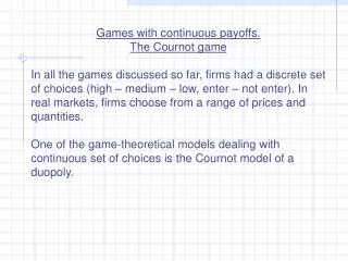
Games with continuous payoffs. The Cournot game

1. Games with continuous payoffs. The Cournot game In all the games discussed so far, firms had a discrete set of choices (high – medium – low, enter – not enter). In real markets, firms choose from a range of prices and quantities. One of the game-theoretical models dealing with continuous set of choices is the Cournot model of a duopoly.

2. “Duopoly” = a market with two firms. The game: Two identical firms producing identical goods enter the same market simultaneously and choose the quantities they are going to produce. Each firm knows what the market demand is but does not know the rival’s choice of quantity. Market demand is Q = 130 – P There are two firms, therefore Q = q1 + q2 Each firm has TCi = 10 qi(i = 1, 2)

3. Firm 1’s profit = P q1 – 10 q1 = (P – 10) q1 = = (130 – q1 – q2– 10) q1 =

4. Firm 1’s profit = P q1 – 10 q1 = (P – 10) q1 = = (130 – q1 – q2 – 10) q1 = (120 – q1 – q2) q1 = = 120 q1 – q12 – q2q1 Firm 1’s profit depends on its own choices AND on Firm 2’s choices; therefore, it is a game. To solve this game, we are going to once again use the best response technique: one firm assumes certain action on the other firm’s part, and finds the best response to that hypothetical action.

5. Let’s assume q2 = 30. What is firm 1’s best response to that? 130 100 DMARKET D1 MC1 10 MR1 30 q1* , our best response

6. The same in mathematical terms: The residual demand for firm 1 is q1 = 100 – P The inverse residual demand is P = 100– q1 Hence MR = 100– 2 q1 If MC = 10, then firm 1’s best response to firm 2’s decision to produce 30 units is MR = MC 100– 2 q1 = 10 90 = 2 q1 q1* = 45

7. The general case: If firm 2 chooses to produce quantity q2, then firm 1’s inverse residual demand is P = (130 – q2)– q1 Hence MR1 = (130 – q2)– 2 q1 If MC = 10, we set MR = MC to get (130 – q2)– 2 q1 = 10, or 2 q1 = 120 – q2, or q1* = 60 – 0.5 q2

8. Alternatively, using differentiation: • The formula for firm 1’s profit is • Π1 = (P – 10) q1 = (130 – q1 – q2 – 10) q1 • If firm 2 produces 30 units, then • Π1 = (90 – q1) q1 = 90 q1 – q12 • We can find our best response by using the profit-maximization approach: • Our control variable is q1. • Take the derivative of our profit with respect to q1, • Set it equal to zero and solve for q1.

9. In the more general case, Π1 = (120 – q2 – q1) q1 = (120 – q2) q1– q12 Even though notation-wise variables q2 and q1 look very similar, we have to keep in mind that Firm 1 has control only over q1 and therefore treats q2 as given, or a constant. All the rules are applied accordingly. (120 – q2) – 2 q1 (120 – q2) – 2 q1 = 0 q1 = 60 – 0.5 q2

10. Either way, we can see that for every q2 chosen by Firm 2, Firm 1 has a unique best response, q1* = 60 – 0.5 q2­ The smaller the q2, the greater the q1* chosen in response. (Makes sense) It is easy to guess that, due to the symmetry of the game, Firm 2’s best response to Firm 1’s choice is q2* = 60 – 0.5 q1 Let us plot the best response functions in the (q1, q2) space.

11. q1*(q2), or BRF of Firm 1 q2 70 60 50 40 30 20 10 The point where strategies (quantity choices) are best responses to each other q2*(q1), or BRF of Firm 2 0 10 20 30 40 50 60 70 80 q1

12. The equilibrium can also be found algebraically, by solving the two best response equations together: q1* = 60 – 0.5 q2 (Eq.1) q2* = 60 – 0.5 q1 (Eq.2) (Since we are looking for best responses of both firms, we can ignore the asterisks or assume all q’s in the equations appear with asterisks.) From (Eq.1), q2 = 120 – 2 q1. Plugging it into (Eq.2) yields 120 – 2 q1 = 60 – 0.5 q1 Rearranging gives 1.5 q1 = 60, or q1 = 40.

13. By plugging q1= 40 into either of the two original equations, we get q2 = 40 (which is not surprising, given the symmetry of the game). We can also calculate resulting equilibrium price(s) and quantities. P = 130 – Q =

14. By plugging q1= 40 into either of the two original equations, we get q2 = 40 (which is not surprising, given the symmetry of the game). We can also calculate resulting equilibrium price(s) and quantities. P = 130 – Q = 130 – (q1 + q2) = $50 Profit of each firm is Π = (P – ATC) ∙ q = (50 – 10) ∙ 40 = $1600

15. Questions for discussion: 1. How will the outcome of the Cournot game change if the firms are no longer identical (the marginal costs of the two firms are different)? 2. How does the outcome of the Cournot game compares to the case when the firms are able to collude?

16. If a monopoly faces demand given by P = 130 – Q, and has MC = $10, then…

17. If a monopoly faces demand given by P = 130 – Q, and has MC = $10, then… TR = P∙Q = (130 – Q) Q = 130 Q – Q2 Marginal Revenue, MR = d(TR) / dQ = 130 – 2 Q, Profit-maximization condition, MR = MC, or 130 – 2 Q = 10 results in 2 Q = 120, or Q = 60 From the demand equation, P = $70, and the resulting profit is (P – ATC) Q

18. If a monopoly faces demand given by P = 130 – Q, and has MC = $10, then… TR = P∙Q = (130 – Q) Q = 130 Q – Q2 Marginal Revenue, MR = d(TR) / dQ = 130 – 2 Q, Profit-maximization condition, MR = MC, or 130 – 2 Q = 10 results in 2 Q = 120, or Q = 60 From the demand equation, P = $70, and the resulting profit is (P – ATC) Q = ($70 - $10) 60 =

19. If a monopoly faces demand given by P = 130 – Q, and has MC = $10, then… TR = P∙Q = (130 – Q) Q = 130 Q – Q2 Marginal Revenue, MR = d(TR) / dQ = 130 – 2 Q, Profit-maximization condition, MR = MC, or 130 – 2 Q = 10 results in 2 Q = 120, or Q = 60 From the demand equation, P = $70, and the resulting profit is (P – ATC) Q = ($70 - $10) 60 = $3600

20. We can summarize our findings in a table. The higher profit earned in the monopoly case explains why firms prefer to collude, or at least to coordinate their prices and outputs in some way.