Download
1 / 20
200 likes | 315 Vues
Learn about robust portfolio modeling for project appraisal under uncertainty, utilizing scenario-based evaluations and decision rules. Discover core indexes, stochastic dominance concepts, and decision-making support for selecting robust project portfolios.

E N D
Robust Portfolio Modeling for Scenario-Based Project Appraisal Juuso Liesiö, Pekka Mild and Ahti Salo Systems Analysis Laboratory Helsinki University of Technology P.O. Box 1100, 02150 TKK, Finland http://www.sal.tkk.fi firstname.lastname@tkk.fi
Project portfolio selection under uncertainty • Robust Portfolio Modeling in multi-attribute evaluation • A subset of projects to be selected subject to resource constraints • Projects evaluated with regard to several attributes • Allows for incomplete information about attribute weights and projects’ scores • Offers robust decision recommendations at project and portfolio level • Core Index values, decision rules • Use of RPM for project selection under uncertainty • Uncertainties captured through scenarios • Projects’ (single-attribute) outcomes known in each scenario • Incomplete information about scenario probabilities • Provides robust decision recommendations • Accounts for the DM’s risk attitude, too
RPM with s cenarios (1/2) • Projects evaluated in each scenario • Projects , outcomes • Scenario probabilities • Project’s expected value • Portfolio is a subset of the available projects • Outcome of portfolio p in ith scenario • Expected portfolio value • A feasible portfolio satisfies a system of linear constraints
RPM with scenarios (2/2) • Problem for a risk neutral DM with known probabilities • Example: n=5 scenarios, m=10 projects
Incomplete information on probabilities (1/2) • Incomplete information on probability estimates • Set of feasible probabilities • Convex polytope bounded by linear constraints • Several probability distributions consistent with this information • E.g. scenario 1 is the most likely out of three:
Dominance concept for a risk neutral DM • Portfolio p dominates p’ if the expected value of p is greater than that of p’ for all feasible probabilities: • Set of non-dominated portfolios • Multi-objective zero-one linear programming problem • MOZOLP algorithms: Bitran (1977), Villareal and Karwan (1980), Deckro and Winkofsky (1983), Liesiö et al. (2005)
Identification of robust projects and portfolios • Core Index of projects • Share of non-dominated portfolios that include the project • CI(x)=1 x is recommended • CI(x)=0 x is not recommended • Examples of decision rules for portfolios • Maximin: ND portfolio with the maximal minimum expected value • Minimax-regret: ND portfolio for which the maximum expected value difference to other feasible portfolios is minimized
Consideration of risk • Accounting for risk aversion • The DM may be interested in portfolios that are dominated in the EV sense • We thus propose a less restrictive approach based on • extention of stochastic dominance concepts to incomplete probability information • introduction of constraints to rule out portfolios which do not satisfy risk requirements • Introduction of risk constraints • E.g., Value-at-Risk (VaR) : The probability of a portfolio value less than must not exceed for any feasible probabilities:
Additional dominance concepts (1/3) • Stochastic dominance • Probability of obtaining a portfolio value at most t: • First degree: • Second degree: • Stochastic dominance checks computationally straightforward • Cumulative distributions are step-functions with steps • Check only required at the extreme points of feasible probability set
Additional dominance concepts (2/3) • Stochastically non-dominated portfolios • A feasible portfolio is non-dominated iff it is not dominated by any other feasible portfolio
Additional dominance concepts (3/3) • Properties • If then has a greater outcome in each scenario • Thus, for any set of feasible probabilities • Therefore • Computation of stochastically non-dominated portfolios • Solve the MOZOLP problem to obtain • Use pair-wise stochastic dominance checks to obtain or
Example (1/3) • Underlying precise probabilities • Approximated by incomplete probability information
Example (2/3) • Maximin , Minimax regret
Example (3/3) • Core Index values for projects • Risk neutrality may be too strong of an assumption • For risk averse DM recommendation can be based on SSD • Projects that can be surely recommended: 1, 5 and 8 • Strong support for project 2 and lack of support for project 3 • Decision rules for portfolios • Maximin: projects 1, 2, 4, 5, 8, 10 • Minimax-regret: • FSD: 1, 5, 7, 8, 9, 10 • SSD: 1, 2, 5, 6, 8, 10 • Expected value: 1,2, 4, 5, 8, 10
Conclusions • RPM for scenario-based project selection • Admits incomplete probability information • Computes all (stochastically) non-dominated portfolios • Indicates projects that are robust choices in view of incomplete information • Decision support • The DM is presented with several portfolios that perform well • Core Indexes support the comparison of projects • Decision rules assist in comparison of portfolios • Current research questions • Consideration of interval-valued multi-attribute project outcomes in scenarios • Explicit modeling of the DM’s risk preferences
References • Liesiö, J., Mild, P., Salo, A., (2005). Preference Programming for Robust Portfolio Modelling and Project Selection, EJOR, (Conditionally Accepted). • Villareal, B., Karwan, M.H., (1981) Multicriteria Integer Programming: A Hybrid Dynamic Programming Recursive Algorithm, Mathematical Programming, Vol. 21, pp. 204-223 • Bitran, G.R., (1977). Linear Multiple Objective Programs with Zero-One Variables, Mathematical Programming, Vol. 13, pp. 121-139. • Decro, R.F., Winkofsky, E.P. (1983). Solving Zero-One Multiple Objective Programs through implicit enumeration, EJOR, Vol. 12, pp. 362-374
Several Time Periods • Model remains linear (cf. CPP) • Each project corresponds to several time-period specific decision variables • Future options depend on decisions in preceding periods • Linear constraints • Resource flow variables transfer leftover resources from one period to another • Maximization of expected value in the last period • Portfolios are compared through their performance in the last time period • LP model includes both continuos and binary variables • Multiple Objective Mixed Zero-One Programming (Mavrotas and Diakoulaki 1998)
Additional dominance concepts • First degree stochastic dominance • Sufficient and necessary condition: • Stochastically non-dominated portfolios
How to model risk attitude? (2/3) • Computation of stochastically non-dominated portfolios • For any set of feasible probabilities since • portfolio p has a greater value than p’ in each scenario • Algorithm • Solve the MOZOLP problem to obtain • Use pair-wise stochastic dominance checks to obtain
How to model risk attitude? (3/3) • Similar treatment for second degree stochastic dominance • Additional information on probabilities or DM’s risk attitude narrows the set of ‘good’ portfolios • For any set of feasible probabilities