Production Theory 1
Production Theory 1. Short-Run v. Long-Run. Fixed input/factor of production: quantity of input is fixed regardless of required output level, e.g. capital or specialized labour Variable input/factor of production: quantity of input used depends on the level of output


Production Theory 1
E N D
Presentation Transcript
Short-Run v. Long-Run • Fixed input/factor of production: quantity of input is fixed regardless of required output level, e.g. capital or specialized labour • Variable input/factor of production: quantity of input used depends on the level of output • Short run: at least one input/factor is fixed • Long run: all inputs/factors are variable
Production Function • A technology is a process by which inputs (e.g. labour and capital) are converted into output. • The output level is denoted by y. • The technology’s production function states the maximum amount of output possible from an input bundle.
Production Function One input Output Level y = f(x) is the production function y’ y’ = f(x’) is the maximum output level obtainable from x’ input units. x’ x Input Level
Technology Set • The collection of all feasible production plans is the technology set.
Technology Set One input Output Level y = f(x) is the production function. y’ y” y” = f(x’) is an output level that is feasible from x’ input units. x’ x Input Level
Technology Set One input Output Level y’ The technologyset y” x’ x Input Level
Technology Set One input Output Level Technicallyefficient plans y’ The technologyset Technicallyinefficientplans y” x’ x Input Level
Technology: Multiple Inputs • What does a technology look like when there is more than one input? • The two input case: Input levels are x1 and x2. Output level is y. • Example of production function is
PREVIEW: ISOQUANT • An isoquant is the set of all combinations of inputs 1 and 2 that are just sufficient to produce a given amount of output. • The slope of the isoquant = the marginal rate of technical substitution (MRTS) = the technical rate of substitution (TRS) • MRTS (TRS): The number of units of K that we can dispose of if one more unit of L becomes available while remaining on the original isoquant.
Technologies with Multiple Inputs • The complete collection of isoquants is the isoquant map. • The isoquant map is equivalent to the production function. • Example
Isoquants with Two Inputs K Y=40 Y=20 L
Isoquants with Two Inputs • Properties Y/K>0, Y/L>0 2Y/K2<0, 2Y/L2<0 Diminishing marginal product (Diminishing marginal utility)
Cobb-Douglas Technology x2 All isoquants are hyperbolic,asymptoting to, but nevertouching any axis. x1
Marginal (Physical) Product • The marginal product of input i is the rate-of-change of the output level as the level of input i changes, holding all other input levels fixed.
Marginal (Physical) Product then the marginal product of input 1 is
Marginal (Physical) Product then the marginal product of input 1 is
Marginal (Physical) Product then the marginal product of input 1 is and the marginal product of input 2 is
Marginal (Physical) Product then the marginal product of input 1 is and the marginal product of input 2 is
Marginal (Physical) Product • The marginal product of input i is diminishing if it becomes smaller as the level of input i increases. That is, if
Technical Rate-of-Substitution The slope is the rate at which input 2 must be given up as input 1’s level is increased so as not to change the output level. The slope of an isoquant is its technical rate-of-substitution. x2 yº100 x1
Technical Rate-of-Substitution • How is a technical rate-of-substitution computed?
Technical Rate-of-Substitution • How is a technical rate-of-substitution computed? • The production function is • A small change (dx1, dx2) in the input bundle causes a change to the output level of
Technical Rate-of-Substitution Along an individual isoquant, dy = 0, therefore the changes dx1 and dx2 must satisfy the following,
Technical Rate-of-Substitution which rearranges to or
Technical Rate-of-Substitution is the rate at which input 2 must be givenup as input 1 increases so as to keepthe output level constant. It is the slopeof the isoquant = MRTS = TRS.