Efficient Subtyping Tests with PQ-Encoding
Efficient Subtyping Tests with PQ-Encoding. Jan Vitek University of Purdue work of: Yoav Zibin and Yossi Gil Technion — Israel Institute of Technology. Outline. Subtyping tests Previous work The PQ Permutation Tree and PQ encoding Results Conclusions & Future Research. Subtyping tests.

Efficient Subtyping Tests with PQ-Encoding
E N D
Presentation Transcript
Efficient Subtyping Tests with PQ-Encoding Jan Vitek University of Purdue work of: Yoav Zibin and Yossi Gil Technion—Israel Institute of Technology
Outline • Subtyping tests • Previous work • The PQ Permutation Tree and PQ encoding • Results • Conclusions & Future Research
Subtyping tests • Is Sylvester a Mammal ? • Catch: • Sylvester is a Feline • a Feline is a Mammal • Given a hierarchy (T,≺) • T is a set of types, |T|=n • ≺ is a partial order over T (reflexive, transitive and anti-symmetric) called subtype relation • Encode the hierarchy so that the query, a≺b, can be answered efficiently. Mammal Feline Canine ?
Efficiency Metrics • Encoding of a hierarchy: a data structure representing the hierarchy which supports subtyping tests. • Metrics: • Test time: answer if a≺b quickly • preferably in constant time • Space: achieve the smallest encoding length • Measured in the average number of bits per type • Encoding creation time • The problem is most interesting for multiple inheritance hierarchies.
Obvious encodings • Binary matrix (BM) • Optimal for arbitrary hierarchies • Test time is constant • For n=5500 the BM size is 3.8MB • Closure-encoding • Stores the ancestors lists • uses M•log n space, but test time is O(log n) • M is the number of both direct and indirect inheritance relations. • DAG-encoding • Stores the parents lists • only m•log n space, but test time is O(n) • m is the number of direct inheritance relations.
Previous Work • Constant encodings for tree hierarchies (single inheritance) • Relative numbering [Schubert ’83] • Cohen's algorithm [Cohen ’91] • Constant encodings for general hierarchies (multiple inheritance) • Packed Encoding (PE) - generalization of Cohen's algorithm [Krall, Vitek and Horspool ’97] (best time results) • Non-constant encodings for general hierarchies • Bit-vectors [Krall, Vitek and Horspool ’97a] (best space results) • And many more, e.g., range-compression, modulation, sparse-terms, and representation using union of interval orders
Relative numbering (for trees only) • Apply postorder numbering • The ordinal of b in the postorder is denoted rb • All descendants of b have consecutive numbers, this interval is denoted [lb ,rb] • a≺blb ≤ra ≤rb
Packed encoding (PE) • Partition the hierarchy into the smallest number of slices • Two types in a slice do not have a common descendant • NP-complete, good heuristic by Vitek et al. 1997 • a≺bra[sb] =idb
Our Technique: PQ encoding (PQE) • Combine the ideas of Relative Numbering with slicing as used in Packed Encoding • Partition the nodes into slices. • Each slice Sihas an ordering πi.of all nodes in the hierarchy. • Slicing property: the descendants of each node b∈Si are consecutive in πi.
Pseudo code for subytping test Procedure IsSub(A,B) // return trueifA < B c slice_of(B) id arrayA[c] [,] interval of descendants of B if (id [,]) return true else return false End The above can be encoded in 4-5 machine instructions
Finding a Good PQ Encoding? • Main objective: minimize the number of slices. • Each slice adds an entry to each one of the arrays. • The main difficulty: the slicing property, i.e., that there is a consecutive ordering of all descendants of nodes in a slice. • Each node in a slice imposes a constraint on the ordering. • Tool: PQ-trees – a data structure which saves all the orderings which satisfy a set of such constraints.
PQ-trees • Invented by Booth and Leuker, 1976 • Used to test for the consecutive 1's property in binary matrices of size rs, in time O(k+r+s) where k is the number of 1's in the matrix. • It is called PQ tree, since it has nodes of two kinds, P- and Q-nodes. • Enabled the first linear time algorithm for recognizing interval graphs (using the maximal cliques matrix) • Used also to recognize (doubly) convex bipartite graphs • Later used for other graph-theoretical problems • on-line planarity testing • maximum planar embeddings • A PQ-tree represents a set of orderings, denoted consistent().
Constructing a PQ-tree • U is the set of all nodes. • A constraint is a set IU which must appear together. • Let 2U be a set of constraints. • Let Π() be the collection of all orderings U such which satisfy all the constraints in . • Theorem (Booth-Leuker (1976)) • For every exists a PQ-tree , and for every exists such that Π()=consistent() • Generating from : • u • u is the universal PQ-tree • reduce(,I) for every I∈ • reduce conducts a bottom-up traversal, at each step applying one of standard eleven PQ-tree transformation
Creation algorithm • 1 ; S[]u • For alla∈T do // Find a PQ-tree consistent with type a • Fors=1,..., do • reduce(S[s],descendants(a)) • exit loop ifreduce succeeded • sas • Ifs= then // Start a new slice • +1 ; S[]u
core height Data-set • 13 non-tree hierarchies used in real life programs • 66-5,438 types (over 18,500 types in total) • PQ works so nicely, since even dense MI hierarchies are tree like in many ways • Average number of parents is always less than 2. • Average number of ancestors can be high (30 in Self) • Height is similar to that of balanced binary tree. • Hierarchies can be broken into a core + bottom trees • A type is in the core if it has a descendant with more than one parent. • The median core size is 21%.
Optimizations • Improving all 3 metrics: test time, space, creation time • Not graph theoretic • Encoding the core, and adding the bottom-trees later • Specialization • Length optimization and pseudo arrays • Heterogeneous encoding • Inlining • Coalescing • This optimization sometimes reduces space, albeit increases test time • The new encoding is called CPQE
Results (Space Metric) • Encoding length of different algorithms • CPQE and BPE are variants of PQE and PE, respectively.
Conclusions & Future Research • PQE improves encoding length, creation time and test time of NHE (details in the paper) • The CPQE variant, tailored for object layout like the one in C++, further reduces the encoding length. • Future work • Incremental encoding
PQ-trees cont. • A PQ-tree has three kinds of a nodes • a leaf which represents a member of a given set U • a Q-node which represents the constraint that all of its children must occur in the order they occur in the tree or in reverse order • a P-node which specifies that its children must occur together, but in any order consistent() frontier()
This interval is denoted [lb,rb] • The ordinal of a in πi is denoted ida[i] • Thus, a≺blb ≤ida[sb] ≤rb a≺blb ≤ida[sb] ≤rb Relative numbering PQE postorder
Previous work - Summary Only for SI Obvious encodings Needs to be compared on the data-set
Bit-vectors • Embeds the hierarchy in the lattice of subsets of {1...k}, each subset is represented as a bit-vector • NP-hard to find minimal k, best heuristic is NHE • a≺bvecbveca =vecb {1,2,3} {1,2,3,6}
≤ ≥ ≺d ≺ π ≤ ∈ • ≤ ≥ ≺d ≺ • ≤ ≥ ≺d ≺ π ≤u ∈
Definitions • ≺d is the transitive reduction of ≺ • ≺ is the transitive closure of ≺d • Formally, a≺d b iff a ≺ b and there is no c such that a ≺ c ≺ b, a≠c≠b. • Also, • ancestors(a)≡{b∈T| a ≺ b}, descendants(a)≡{b∈T| b ≺ a} • parents(a)≡{b∈T| a ≺d b}, children(a)≡{b∈T| b ≺d a} • roots≡{a∈T| parents(a)=∅}, leaves≡{a∈T| children(a)=∅} • level(a)≡1+max{level(b)| b∈parents(a)} • Single inheritance (SI) vs. multiple inheritance (MI) • In SI, for each a∈T, |parents(a)|≤1
Cohen's algorithm • Partition the hierarchy into levels • a≺blb≤ la and ra[lb] =idb • lbis level(b), idb is a unique identifier within the level
Range compression • Apply postorder on some spanning forest • a ≺ b lb[i]≤ida ≤rb[i] , for some i {1,2,3} {2,5,6}
Optimizations • Creation time • Encoding the core, and inserting the bottom-trees later • Encoding length • Length optimization • reduces the range needed for the ids. Thus, all slices (except the first) only uses a single byte. • Heterogeneous encoding • uses BM representation for slices whose size is smaller than 8. • Specialization • Emitting values which depend only on the supertype into the test code, e.g., lb and rb. • Also improves test time (saves load instructions).
Inlining optimization • Uses the freedom the compiler have in placing the runtime representation of the types • The first slice is inlined • Instead of using ida[1] we use the pointer to the runtime representation • Reduces 16 bits from the encoding length • Saves one load if the supertype is from the first slice • The first slice constitutes 90% of the types • Using this technique in relative-numbering reduces the encoding length to zero.
Coalesced PQ-encoding (CPQE) • When C++ had only SI, the runtime information was stored before the VTBL • In MI there could be many VTBLs • Implementers can either duplicate or share • Sharing is done by another level of indirection • In CPQE types can share their id array • Since the first slice was inlined, some arrays can be coalesced • The number of distinct arrays is always lower than the size of the core
Results cont. • Encoding creation time in milliseconds • (C)PQE on 266 Mhz Pentium II • NHE on 500 Mhz 21164 Alpha • (B)PE on 750 Mhz Pentium~III, user time in Linux
2-Dim encoding • Idea: embed the hierarchy in the plane • If not possible, use multiple slices a≺b Xa[sb]≥Xb[sb] and Ya[sb]≥Yb[sb] 2-Dim encoding using one slice
Encoding creation • A slice S has a pseudo 2-dimensional embedding if we can embed the hierarchy so that queries a ≺ b, b∈S, are answered correctly • Theorem: A slice S has a pseudo 2-dimensional embedding iff dim(HS)=2