Econometric Forecasting with Linear Regression
750 likes | 913 Vues
Econometric Forecasting with Linear Regression. A Brief Introduction. I. Fundamental Concepts. Data (variables). Can be in three forms:

Econometric Forecasting with Linear Regression
E N D
Presentation Transcript
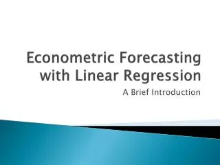
Econometric Forecasting with Linear Regression A Brief Introduction
I. Fundamental Concepts • Data (variables). Can be in three forms: • Interval – There is a common scale to measure the variable, so that a value of two is actually twice a value of one. Examples: % of vote, degrees Fahrenheit, number killed, duration of regime, number of soldiers, GDP • Ordinal – There is a rank-ordering to the variable, so 2 > 1, but the scale varies so that 2 is not exactly twice one. Examples: Yes/No variables, how close a bill is to passage (no houses, one house, both houses, signature), war outcomes (win, lose, or draw) • Nominal – There are numbers, but they are completely arbitrary. Examples: country codes, leader names, strategy choices, apples and oranges.
B. Dependent Variable: What you are trying to predict • Examples include % of the two-party Presidential vote, % seats held by Dems, war/non-war, political (in)stability, etc. • Easiest to have a continuous (interval) DV, but techniques exist for all three types
C. Independent Variables: What variables predict the DV • Can be either interval or ordinal. So… • Transform nominal into ordinal. Example: Is this country the US? A nominal variable (USA) becomes an ordinal one (Yes or No). • Again, examples in syllabus
D. Correlation • Positive (or direct) correlation: the values of the IV and DV move up and down together (poverty and crime, CO2 and global temperature, drug addiction and prostitution, geographic proximity and conflict)
D. Correlation • Positive (or direct) correlation: the values of the IV and DV move up and down together (poverty and crime, CO2 and global temperature, drug addiction and prostitution, geographic proximity and conflict) • Negative (or inverse): The values of the IV and DV move in opposite directions (alcohol and coordination, democracy and interstate conflict, war and development)
D. Correlation • Positive (or direct) correlation: the values of the IV and DV move up and down together (poverty and crime, CO2 and global temperature, drug addiction and prostitution, geographic proximity and conflict) • Negative (or inverse): The values of the IV and DV move in opposite directions (alcohol and coordination, democracy and interstate conflict, war and development) • Conditional: Direction depends on the value of some other variable
4. Correlation ≠ Causation: Coincidence and Omitted Variables
E. Example: Forecasting Political Stability with Five Variables Dependent Variable Independent Variables Statistical Relationships
II. Modeling Relationships • Simplest tool: the scatterplot or scatter diagram. Example from medicine:
Example • A researcher believes that there is a linear relationship between BMI (Kg/m2) of pregnant mothers and the birth-weight (BW in Kg) of their newborn • The following data set provide information on 15 pregnant mothers who were contacted for this study
BMI (Kg/m2) Birth-weight (Kg) 20 2.7 30 2.9 50 3.4 45 3.0 10 2.2 30 3.1 40 3.3 25 2.3 50 3.5 20 2.5 10 1.5 55 3.8 60 3.7 50 3.1 35 2.8
Scatter Diagrams / Scatterplots • Scatter diagram plots bivariateobservations (X, Y) BMI (the IV) is X and birthweight (the DV) is Y • Y is the dependentvariable (Dependent goes Down the side) • X is the independent variable (goes across the graph)
B. Interpreting Scatterplots • People tend to mentally fit a line or curve to describe the shape of the scatterplot • Examples:
Linear Correlation Strong relationships Weak relationships Y Y X X Y Y X X
Linear (lack of) Correlation No relationship Y X Y X
Curvilinear Correlation Linear relationships Curvilinear relationships Y Y X X Y Y X X
C. What does the line mean? • Intended to simplify relationship. The line is ultimately an estimate, usually known to be wrong (but close enough to be useful) • Line is probabilistic, not deterministic – otherwise it would perfectly pass through every point on the scatterplot • = key difference between predicting politics and predicting planetary orbits. Kepler’s equations are deterministic, but econometric models are probabilistic
D. Problem: How do we draw the “right” line? • Sample scatterplot: Y 60 40 20 0 X 0 20 40 60
Thinking Challenge How would you draw a line through the points? How do you determine which line ‘fits best’?
Thinking Challenge How would you draw a line through the points? How do you determine which line ‘fits best’?
Thinking Challenge How would you draw a line through the points? How do you determine which line ‘fits best’?
Thinking Challenge How would you draw a line through the points? How do you determine which line ‘fits best’?
Thinking Challenge How would you draw a line through the points? How do you determine which line ‘fits best’?
Thinking Challenge How would you draw a line through the points? How do you determine which line ‘fits best’?
Thinking Challenge How would you draw a line through the points? How do you determine which line ‘fits best’?
E. Solution: Regression • Regression = using an equation to find the line (or curve) that most closely fits the data
1. Linear Regression Model • a.Relationship Between Variables Is a Linear Function Coefficient of X, or Slope Constant, or Y-Intercept Random Error Y X 0 1 Dependent Variable Independent (Explanatory or Control) Variable
Does this equation look a bit familiar? • It should….
b. Linear Equations High School Teacher
c. Quick math review • As you remember from high school math, the basic equation of a line is given by y=mx+b where m is the slope and b is the y-intercept • One definition of m is that for every one unit increase in x, there is an m unit increase in y • One definition of b is the value of y when x is equal to zero
Sample Scatterplot • Look at the data in this picture • Does there seem to be a correlation (linear relationship) in the data? • Is the data perfectly linear? • Could we fit a line to this data?
2. What is linear regression? • Linear regression tries to find the best line (curve) to fit the data • The equation of the line is • The method of finding the best line (curve) is least squares, which minimizes the sum of the distance from the line for each of points
3. Ordinary Least Squares (OLS): The most common form of linear regression • Find the values of b that minimize the squared vertical distance from the line to each of the point. This is the same as minimizing the sum of the ei2 • Why minimize squared errors? ‘Best Fit’ Means Difference Between Actual Y Values & Predicted Y Values Are a Minimum But Positive Differences Offset Negative! (errors of 10 and -10 add to zero) squaring errors solves the problem: 10 * 10 = 100 and -10 * -10 also = 100.
c. Least Squares Graphically: Predicted Values of Y vs. Actual Values of Y For each observation i, the equation is merely an estimate, not the actual value. There are errors (εi), and the line minimizes the sum of ε12, ε22, ε32, ε42, ε52, and so on.
d. Recap: Interpreting the Linear Regression Formula 47 • Regression Formula: Y = a + bX, Y = α + βX, Y = α + β1X1, Y = β0 + β1X1, etc all are the same formula! • Y = the predicted value of the dependent variable (its estimated mean given X) • a(or alpha: α, or beta-zero: β0) = the Y intercept, or the value of Y when X = 0 (constant) • b(or beta: β) = the regression coefficient, the slope of the regression line, or the amount of change produced in Y by a unit change in X • Positive sign of regression coefficient: positive direction of association • Negative sign of regression coefficient: negative direction of association • X = the value of the independent variable
Example • What is: • Y? • X? • β1? • β0?
e. Multivariate Linear Regression 49 • Typical formula: Y = β0 + β1X1 + β2X2 + β3X3, etc. • DV, constant haven’t changed • But now there are several independent variables • Each IV has its own coefficient. So the first X may be positively related to Y, while the others might be negatively related to Y. • Could plot the effect of any one independent variable on Y as a line, but can no longer plot the whole equation since there are now as many dimensions as there are independent variables (plus one, for Y). • Multivariate regression is best interpreted by consulting tables of coefficients, evaluating the effect of each X separately (i.e. all else being equal)
F. Other statistics generated by linear regression 1. R2 : Proportion of the variation in the dependent variable (Y ) that is explained by the independent variable (X) R2 =Explained variation/Total variation Ranges between 0 (no reduction in error) and 1 (no errors remain – the model perfectly predicts the dependent variable) R2 is a comparative measure – it compares the amount of error made by the linear regression to the amount of error made by guessing the mean (average) value of Y for every case (e.g. Y = 12 for every case) 50