Tree-Structured Indexes
Learn about B+-tree index files as an alternative to indexed-sequential files, their advantages and disadvantages, node structures, search mechanisms, and practical implementations, including insertion methods and tree growth scenarios.

Tree-Structured Indexes
E N D
Presentation Transcript
Tree-Structured Indexes Content based on Chapter 10 Database Management Systems, (3rd Edition), by Raghu Ramakrishnan and Johannes Gehrke. McGraw Hill, 2003
B+-Tree Index Files B+-tree indices are an alternative to indexed-sequential files. • Disadvantage of indexed-sequential files • performance degrades as file grows, since many overflow blocks get created. • Periodic reorganization of entire file is required. • Advantage of B+-treeindex files: • automatically reorganizes itself with small, local, changes, in the face of insertions and deletions. • Reorganization of entire file is not required to maintain performance. • (Minor) disadvantage of B+-trees: • extra insertion and deletion overhead, space overhead. • Advantages of B+-trees outweigh disadvantages • B+-trees are used extensively
B+-Tree Node Structure • Typical node • Ki are the search-key values • Pi are pointers to children (for non-leaf nodes) or pointers to records or buckets of records (for leaf nodes). • The search-keys in a node are ordered K1 <K2 <K3 <. . .<Kn–1 (Initially assume no duplicate keys, address duplicates later)
Leaf Nodes in B+-Trees Properties of a leaf node: • For i = 1, 2, . . ., n–1, pointer Pi points to a file record with search-key value Ki, • If Li, Lj are leaf nodes and i < j, Li’s search-key values are less than or equal to Lj’s search-key values • Pn points to next leaf node in search-key order
Index Entries (Direct search) Data Entries ("Sequence set") B+ Tree: Most Widely Used Index • Insert/delete at log F N cost; keep tree height-balanced. (F = fanout, N = # leaf pages) • Minimum 50% occupancy (except for root). Each node contains d <= m <= 2d entries. The parameter d is called the order of the tree. • Supports equality and range-searches efficiently.
Observations about B+-trees • Since the inter-node connections are done by pointers, “logically” close blocks need not be “physically” close. • The non-leaf levels of the B+-tree form a hierarchy of sparse indices. • The B+-tree contains a relatively small number of levels • Level below root has at least 2* n/2 values • Next level has at least 2* n/2 * n/2 values • .. etc. • If there are K search-key values in the file, the tree height is no more than logn/2(K) • thus searches can be conducted efficiently. • Insertions and deletions to the main file can be handled efficiently, as the index can be restructured in logarithmic time.
Queries on B+-Trees • Find record with search-key value V. • C=root • While C is not a leaf node { • Let i be least value s.t. V Ki. • If no such exists, set C = last non-null pointer in C • Else { if (V= Ki ) Set C = Pi +1 else set C = Pi} } • Let i be least value s.t. Ki = V • If there is such a value i, follow pointer Pito the desired record. • Else no record with search-key value k exists.
Queries on B+-Trees (Cont.) • If there are K search-key values in the file, the height of the tree is no more than logn/2(K). • A node is generally the same size as a disk block, typically 4 kilobytes • and n is typically around 100 (40 bytes per index entry). • With 1 million search key values and n = 100 • at most log50(1,000,000) = 4 nodes are accessed in a lookup. • Contrast this with a balanced binary tree with 1 million search key values — around 20 nodes are accessed in a lookup • above difference is significant since every node access may need a disk I/O, costing around 20 milliseconds
Example B+ Tree • Search begins at root, and key comparisons direct it to a leaf. • Search for 5*, 15*, all data entries >= 24* ... Root 30 13 17 24 39* 3* 5* 19* 20* 22* 24* 27* 38* 2* 7* 14* 16* 29* 33* 34* • Based on the search for 15*, we know it is not in the tree!
B+ Trees in Practice • Typical order: 100. Typical fill-factor: 67%. • average fanout = 133 • Typical capacities: • Height 4: 1334 = 312,900,700 records • Height 3: 1333 = 2,352,637 records • Can often hold top levels in buffer pool: • Level 1 = 1 page = 8 Kbytes • Level 2 = 133 pages = 1 Mbyte • Level 3 = 17,689 pages = 133 MBytes
Inserting a Data Entry into a B+ Tree • Find correct leaf L. • Put data entry onto L. • If L has enough space, done! • Else, must splitL (into L and a new node L2) • Redistribute entries evenly, copy upmiddle key. • Insert index entry pointing to L2 into parent of L. • This can happen recursively • To split index node, redistribute entries evenly, but push upmiddle key. (Contrast with leaf splits.) • Splits “grow” tree; root split increases height. • Tree growth: gets wideror one level taller at top.
Example B+ Tree - Inserting 15* Root 30 24 13 17 39* 22* 24* 27* 38* 3* 5* 19* 20* 29* 33* 34* 2* 7* 14* 16* 16* 14* 15* Dose not violates the 50% rule
Example B+ Tree - Inserting 8* Root 30 24 13 17 39* 22* 24* 27* 38* 3* 5* 19* 20* 29* 33* 34* 2* 7* 14* 16* 3* 5* 8* 2* 7* Violates the 50% rule, split the leaf.
Example B+ Tree - Inserting 8* Violates the 50% rule, split the internal node. Root 5 30 24 13 17 39* 22* 24* 27* 38* 3* 19* 20* 29* 33* 34* 2* 14* 16* 7* 8* 5*
Example B+ Tree After Inserting 8* Root 17 24 5 13 30 39* 2* 3* 5* 7* 8* 19* 20* 22* 24* 27* 38* 29* 33* 34* 14* 16* • Notice that root was split, leading to increase in height. • In this example, we can avoid split by re-distributing entries; however, this is usually not done in practice.
Entry to be inserted in parent node. (Note that 17 is pushed up and only 17 this with a leaf split.) 5 13 24 30 Inserting 8* into Example B+ Tree Entry to be inserted in parent node. (Note that 5 is s copied up and • Observe how minimum occupancy is guaranteed in both leaf and index pg splits. • Note difference between copy-up and push-up; be sure you understand the reasons for this. 5 continues to appear in the leaf.) 3* 5* 2* 7* 8* appears once in the index. Contrast
Deleting a Data Entry from a B+ Tree • Start at root, find leaf L where entry belongs. • Remove the entry. • If L is at least half-full, done! • If L has only d-1 entries, • Try to re-distribute, borrowing from siblings (adjacent nodes with same parent as L). • If re-distribution fails, mergeL and sibling. • If merge occurred, must delete entry (pointing to L or sibling) from parent of L. • Merge could propagate to root, decreasing height.
Example Tree (including 8*) Delete 19* and 20* ... Root 17 24 30 5 13 39* 2* 3* 19* 20* 22* 24* 27* 38* 5* 7* 8* 29* 33* 34* 14* 16*
Example Tree (including 8*) After 19* is Deleted. Delete 20 • Deleting 19* is easy. Root 17 24 30 5 13 39* 2* 3* 20* 22* 24* 27* 38* 5* 7* 8* 29* 33* 34* 14* 16*
Example Tree (including 8*) Delete 20* • Underflow! → Redistribute. Root 17 24 30 5 13 39* 2* 3* 24* 27* 38* 5* 7* 8* 29* 33* 34* 14* 16* 22* Violates the 50% rule
Example Tree After (Inserting 8*, Then) Deleting 19* and 20* ... • Deleting 20* is done with re-distribution. Notice how the lowest key is copied up. Root 17 27 5 13 30 39* 2* 3* 5* 7* 8* 22* 24* 27* 29* 38* 33* 34* 14* 16*
... And Then Deleting 24* Root 17 27 5 13 30 39* 2* 3* 5* 7* 8* 22* 24* 27* 29* 38* 33* 34* 14* 16* • Underflow! • Can we do redistribution? • MERGE!
... And Then Deleting 24* • Must merge. • Observe `toss’ of index entry (on right), and `pull down’ of index entry (below). 30 39* 22* 27* 38* 29* 33* 34* Root 5 13 17 30 3* 39* 2* 5* 7* 8* 22* 38* 27* 33* 34* 14* 16* 29*
2* 3* 5* 7* 8* 39* 17* 18* 38* 20* 21* 22* 27* 29* 33* 34* 14* 16* Example of Non-leaf Re-distribution • Tree is shown below during deletion of 24*. • In contrast to previous example, can re-distribute entry from left child of root to right child. Root 22 30 17 20 5 13
After Re-distribution • Intuitively, entries are re-distributed by `pushingthrough’ the splitting entry in the parent node. • It suffices to re-distribute index entry with key 20. Root 20 30 5 13 22 17 2* 3* 5* 7* 8* 39* 17* 18* 38* 20* 21* 22* 27* 29* 33* 34* 14* 16*
After Re-distribution • Intuitively, entries are re-distributed by `pushingthrough’ the splitting entry in the parent node. • We’ve re-distributed 17 as well for illustration. Root 17 22 30 5 13 20 2* 3* 5* 7* 8* 39* 17* 18* 38* 20* 21* 22* 27* 29* 33* 34* 14* 16*
Indexing Strings • Variable length strings as keys • Variable fanout • Use space utilization as criterion for splitting, not number of pointers • Prefix compression • Key values at internal nodes can be prefixes of full key • Keep enough characters to distinguish entries in the subtrees separated by the key value • E.g. “Silas” and “Silberschatz” can be separated by “Silb” • Keys in leaf node can be compressed by sharing common prefixes
Bulk Loading and Bottom-Up Build • Inserting entries one-at-a-time into a B+-tree requires 1 IO per entry • assuming leaf level does not fit in memory • can be very inefficient for loading a large number of entries at a time (bulk loading) • Efficient alternative 1: • sort entries first • insert in sorted order • insertion will go to existing page (or cause a split) • much improved IO performance, but most leaf nodes half full • Efficient alternative 2: Bottom-up B+-tree construction • As before sort entries • And then create tree layer-by-layer, starting with leaf level • Implemented as part of bulk-load utility by most database systems
3* 6* 9* 10* 11* 12* 13* 23* 31* 36* 38* 41* 44* 4* 20* 22* 35* Bulk Loading of a B+ Tree • If we have a large collection of records, and we want to create a B+ tree on some field, doing so by repeatedly inserting records is very slow. • Bulk Loadingcan be done much more efficiently. • Initialization: Sort all data entries, insert pointer to first (leaf) page in a new (root) page. Root Sorted pages of data entries; not yet in B+ tree
3* 6* 9* 10* 11* 12* 13* 23* 31* 36* 38* 41* 44* 4* 20* 22* 35* Bulk Loading of a B+ Tree Root Sorted pages of data entries; not yet in B+ tree 6
3* 6* 9* 10* 11* 12* 13* 23* 31* 36* 38* 41* 44* 4* 20* 22* 35* Bulk Loading of a B+ Tree Root Sorted pages of data entries; not yet in B+ tree 6 10
Bulk Loading (Contd.) Root 10 20 • Index entries for leaf pages always entered into right-most index page just above leaf level. When this fills up, it splits. (Split may go up right-most path to the root.) • Much faster than repeated inserts, especially when one considers locking! Data entry pages 6 12 23 35 not yet in B+ tree 3* 6* 9* 10* 11* 12* 13* 23* 31* 36* 38* 41* 44* 4* 20* 22* 35* Root 20 10 Data entry pages 35 not yet in B+ tree 6 23 12 38 3* 6* 9* 10* 11* 12* 13* 23* 31* 36* 38* 41* 44* 4* 20* 22* 35*
Range Searches • ``Find all students with gpa > 3.0’’ • If data is in sorted file, do binary search to find first such student, then scan to find others. • Cost of binary search can be quite high. • Simple idea: Create an `index’ file. Index File kN k2 k1 Data File Page N Page 3 Page 1 Page 2 • Can do binary search on (smaller) index file!
Animation • https://www.cs.usfca.edu/~galles/visualization/BPlusTree.html